- Wave function
-
Not to be confused with the related concept of the Wave equation
 Some trajectories of a harmonic oscillator (a ball attached to a spring) in classical mechanics (A-B) and quantum mechanics (C-H). In quantum mechanics (C-H), the ball has a wave function, which is shown with real part in blue and imaginary part in red. The trajectories C,D,E,F, (but not G or H) are examples of standing waves, (or "stationary states"). Each standing-wave frequency is proportional to a possible energy level of the oscillator. This "energy quantization" does not occur in classical physics, where the oscillator can have any energy.
Quantum mechanics

Introduction
Mathematical formulationsFundamental conceptsQuantum state · Wave function
Superposition · Entanglement
Complementarity · Duality
Uncertainty · Measurement
Exclusion · Decoherence
Ehrenfest theorem
Tunnelling · NonlocalityExperimentsDouble-slit · Davisson–Germer
Stern–Gerlach · Bell's inequality
Popper · Schrödinger's cat
Elitzur–Vaidman bomb tester
Quantum eraser
Delayed choice quantum eraser
Wheeler's delayed choiceFormulationsEquationsInterpretationsde Broglie–Bohm
Consciousness-caused
Consistent histories · Copenhagen
Ensemble · Hidden variables
Many-worlds · Objective collapse
Pondicherry · Quantum logic
Relational · Stochastic
TransactionalScientistsBell · Bohm · Bohr · Born · Bose
de Broglie · Dirac · Ehrenfest
Everett · Feynman · Heisenberg
Jordan · Kramers · von Neumann
Pauli · Planck · Schrödinger
Sommerfeld · Wien · WignerA wave function or wavefunction is a probability amplitude in quantum mechanics describing the quantum state of a particle and how it behaves. Typically, its values are complex numbers and, for a single particle, it is a function of space and time. The laws of quantum mechanics (the Schrödinger equation) describe how the wave function evolves over time. The wave function behaves qualitatively like other waves, like water waves or waves on a string, because the Schrödinger equation is mathematically a type of wave equation. This explains the name "wave function", and gives rise to wave-particle duality.
The most common symbols for a wave function are ψ or Ψ (lower-case and capital psi).
Although ψ is a complex number, |ψ|2 is real, and corresponds to the probability density of finding a particle in a given place at a given time, if the particle's position is measured.
The SI units for ψ depend on the system. For one particle in three dimensions, its units are m–3/2. These unusual units are required so that an integral of |ψ|2 over a region of three-dimensional space is a unitless probability (i.e., the probability that the particle is in that region). For different numbers of particles and/or dimensions, the units may be different.
The wave function is absolutely central to quantum mechanics: it makes the subject what it is. Also; it is the source of the mysterious consequences and philosophical difficulties in what quantum mechanics means in nature, and even how nature itself behaves at the atomic scale and beyond - which continue in debate to this day.
Historical background
Calculus and linear algebra: wave and matrix mechanics
In the 1920s and 1930s, there were two divisions (so to speak) of theoretical physicists who simultaneously founded quantum mechanics: one for calculus and one for linear algebra. Those who used the techniques of calculus included Louis de Broglie, Erwin Schrödinger, Paul Dirac, Hermann Weyl, Oskar Klein, Walter Gordon, Douglas Hartree and Vladimir Fock. This hand of quantum mechanics became known as "wave mechanics". Those who applied the methods of linear algebra included Werner Heisenberg, Max Born, Wolfgang Pauli and John Slater. This other hand of quantum mechanics came to be called "matrix mechanics". Schrödinger was one who subsequently showed that the two approaches were equivalent. [1] In each case, the wavefunction was at the centre of attention in two forms, giving quantum mechanics its ubiquitous unity.
Introduction of wave functions
De Broglie could be considered the founder of the wave model in 1925, due to his symmetric relation between momentum and wavelength: the De Broglie equation. Schrödinger searched for an equation that would describe these waves, and was the first to construct and publish an equation for which the wave function satisfied in 1926, based on classical energy conservation. Indeed it is now called the Schrödinger equation.
Interpretation and acceptance
However, no-one, even Schrödinger and De Broglie, were clear on how to interpret it. What did this function mean? Around 1924–27, Born, Heisenberg, Bohr and others provided the perspective of probability amplitude. This is the Copenhagen interpretation of quantum mechanics. There are many other interpretations of quantum mechanics, but this is considered the most important - since quantum calculations can be understood.
Applications and approximations
In 1927, Hartree and Fock made the first step in an attempt to solve the N-body wave function, and developed the self-consistency cycle: an iterative algorithm to approximate the solution. Now it is also known as the Hartree–Fock method[2]. The Slater determinant and permanent (of a matrix) was part of the method, provided by Slater.
Relativistic wave functions
Interestingly, Schrödinger did encounter an equation for which the wave function satisfied relativistic energy conservation before he published the non-relativistic one, but it lead to unacceptable consequences for that time so he discarded it. [3]In 1927, Klien, Gorden and Fock also found it, but taking a step further: enmeshed the electromagnetic interaction into it and proved it was Lorentz-invariant. De Broglie also arrived at exactly the same equation in 1928. This wave equation is now known most commonly as the Klein–Gordon equation [4].
By 1928 Dirac deduced his equation from the first successful unified combination of special relativity and quantum mechanics to the electron - the Dirac equation. He found an unusual character of the wavefunction for this equation: it was not a single complex number, but a spinor[5]. Spin automatically entered into the properties of the wavefunction. Although there were problems; Dirac was capable of resolving them. Around the same time Weyl also found his relativistic equation, which also had spinor solutions.
Later other wave equations were developed: see Relativistic wave equations for further information.
Definition (single spin-0 particle in one spatial dimension)
Wavefunctions as multi-variable functions - analytical calculus formalism
Multivariable calculus and analysis (study of functions, change etc.) can be used to represent the wavefunction in a number of situations. Superficially, this formalism is simple to understand for the following reasons.
- It is more directly intiutive to have probability amplitudes as functions of space and time. At every position and time coordinate, the probability amplitude has a value by direct calculation.
- Functions can easily describe wave-like motion, using periodic functions, and Fourier analysis can be readily done.
- Functions are easy to produce, visualize and interpret, due to the pictorial nature of the graph of a function (i.e. curves, contours, surfaces). When the situation is in a high number of dimensions (say 3) - it is possible to analyse the function in a lower dimensional slice (say 2) or contour plots of the function to determine the behaviour of the system within that confined region.
Although these functions are continuous - they are not deterministic; but probability distributions. Perhaps oddly, it this approach is not the most general way to represent probability amplitudes. The more advanced techniques use linear algebra (the study of vectors, matrices, etc.) and more generally still; abstract algebra (algebraic structures, generalizations of Euclidean spaces etc.).
Position-space wavefunction
For now, consider the simple case of a single particle, without spin, in one spatial dimension. (More general cases are discussed below). The state of such a particle is completely described by its wave function:
- Ψ(x,t),
where x is position and t is time. This function is complex-valued, meaning that Ψ(x,t) is a complex number.
If the particle's position is measured, its location is not deterministic, but is described by a probability distribution. The probability that its position x will be in the interval [a,b] (meaning a ≤ x ≤ b) is:
where t is the time at which the particle was measured. In other words, | Ψ(x,t) | 2 is the probability density that the particle is at x, rather than some other location.
This leads to the normalization condition:
 ,
,
because if the particle is measured, there is 100% probability that it will be somewhere.
Momentum-space wavefunction
Main article: Momentum spaceThe particle also has a wave function in momentum space:
- Φ(p,t)
where p is the momentum in one dimension, which can be any value from
 to
to  , and t is time. If the particle's momentum is measured, the result is not deterministic, but is described by a probability distribution:
 ,
,
analogous to the position case. The position-space and momentum-space wave functions are Fourier transforms of each other, therefore both contain the same information, and either one alone is sufficient to calculate any property of the particle. For one-dimension:[6]
Sometimes the wave-vector k is used in place of momentum p, since they are related by the de Broglie relation
and the equivalent space is referred to as k-space. Again it makes no difference which is used since p and k are equivalent - up to a constant. In practice, the position-space wavefunction is used much more often than the momentum-space wavefunction.
 Wave-particles "stationary".
 Wave-particles travelling.Interpretation of wave function for one spin-0 particle in one dimension. The wavefunctions shown are continuous, finite, single-valued and normalized. The colour opacity (%) of the particles corresponds to the probability density (which can measure in %) of finding the particle at the points on the x-axis.
Wave functions as an abstract vector space - linear/abstract algebra formalism
The set of all possible wave functions (at any given time) forms an abstract mathematical vector space. Specifically, the entire wave function is treated as a single abstract vector:
(
 is a column vector written in bra-ket notation). The statement that "wave functions form an abstract vector space" simply means that it is possible to add together different wave functions, and multiply wave functions by complex numbers (see vector space for details). (Technically, because of the normalization condition, wave functions form a projective space rather than an ordinary vector space.) This vector space is infinite-dimensional, because there is no finite set of functions which can be added together in various combinations to create every possible function. Also, it is a Hilbert space, because the inner product of wave functions Ψ1(x) and Ψ2(x) can be defined as
where * denotes complex conjugate.
There are several advantages to understanding wave functions as elements of an abstract vector space:
- All the powerful tools of linear algebra can be used to manipulate and understand wave functions. For example:
- Linear algebra explains how a vector space can be given a basis, and then any vector can be expressed in this basis. This explains the relationship between a wave function in position space and a wave function in momentum space, and suggests that there are other possibilities too.
- Bra-ket notation can be used to manipulate wave functions.
- The idea that quantum states are vectors in a Hilbert space is completely general in all aspects of quantum mechanics and quantum field theory, whereas the idea that quantum states are complex-valued "wave" functions of space is only true in certain situations.
Introduction to vector formalism
Given an isolated physical system, the allowed states of this system (i.e. the states the system could occupy without violating the laws of physics) are part of a Hilbert space H. Some properties of such a space are
- If and
 are two allowed states, then
-
- is also an allowed state, provided
 . (This condition is due to normalisation, see below.)
- There is always an orthonormal basis of allowed states of the vector space H.
Physically, the nature of the inner product is dependent on the basis in use, becuase the basis is chosen to reflect the quantum state of the system.
When the basis is a countable set
 and orthonormal, that is
then an arbitrary vector
can be expressed aswhere the components are the (complex) numbers
 This wave function is known as a descrete spectrum, since the bases are descrete.
When the basis is an uncountable set, the orthonormality condition holds similarly,
then an arbitrary vector
can be expressed aswhere the components are the functions
 This wave function is known as a continuous spectrum, since the bases are continuous.
Paramount to the analysis is the Kronecker delta, δij, and the Dirac delta function,
 , since the bases used are orthonormal. More detailed discussion of wave functions as elements of vector spaces is below, following further definitions.
Definition (other cases)
Many spin-0 particles in one spatial dimension
The wavefunction can be generalized to incorporate N particles in one dimension:
 ,
,
The probability that particle 1 is in an x-interval R1 = [a1,b1] and particle 2 in interval R2 = [a2,b2] etc, up to particle N in interval RN = [aN,bN], all measured simultaneously at time t, is given by:
The normalization condition becomes:
 .
.
In each case, there are N one-dimensional integrals, one for each particle.
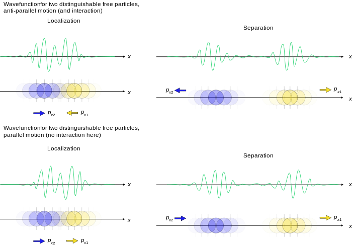 Visulization of the wavefunction for two spin-0 particles, in one dimension. Above: The two particles interact, then recoil from each other with 100% certainty. This situation occurs in quantum entanglement. Below: The particles are simply travelling.
One spin-0 particle in three spatial dimensions
Position space wavefunction
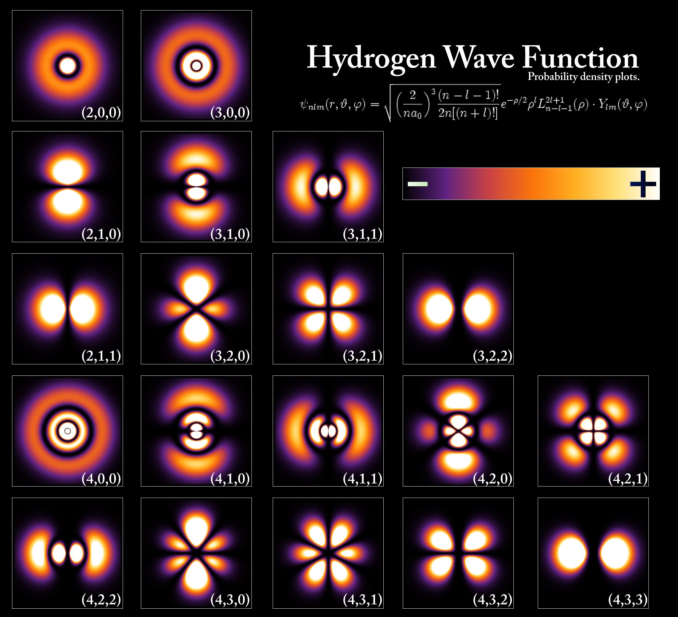
 The electron probability density for the first few hydrogen atom electron orbitals shown as cross-sections. These orbitals form an orthonormal basis for the wave function of the electron. Different orbitals are depicted with different scale.
The position-space wave function of a single particle in three spatial dimensions is similar to the case of one spatial dimension above:
where r is the position in three-dimensional space (r is short for (x,y,z)), and t is time. As always
 is a complex number. If the particle's position is measured at time t, the probability that it is in a region R is:
(a three-dimensional integral over the region R, with differential volume element d3r, also written "dV" or "dx dy dz"). The normalization condition is:
where
 is all of three-dimensional space.
Momentum space wavefunction
There is a corresponding momentum space wavefunction for three-dimensions also:
where p is the momentum in 3-dimensional space, and t is time. This time there are three components of momentum which can have values
to in each direction, in Cartesian coordinates x, y, z.The probability of measuring the momentum components px between a and b, py between c and d, and pz between e and f, is given by:
hence the normalization:
The generalization of the previous Fourier transform is [7]
Many spin-0 particles in three spatial dimensions
When there are many particles, there is only one wave function, not a separate wave function for each particle. The fact that one wave function describes many particles is what makes quantum entanglement and the EPR paradox possible. The position-space wave function for N particles is written:[8]
where ri is the position of the ith particle in three-dimensional space, and t is time. If the particles' positions are all measured simultaneously at time t, the probability that particle 1 is in region R1 and particle 2 is in region R2 and so on is:
The normalization condition is:
(altogether, this is 3N one-dimensional integrals).
In quantum mechanics there is a fundamental distinction between identical particles and distinguishable particles. For example, any two electrons are fundamentally indistinguishable from each other; the laws of physics make it impossible to "stamp an identification number" on a certain electron to keep track of it.[9] This translates to a requirement on the wavefunction: For example, if particles 1 and 2 are indistinguishable, then:
where the + sign is required if the particles are bosons, and the – sign is required if they are fermions. More exactly stated:
where s = spin quantum number,
- integer for bosons:

- and half-integer for fermions:

The wavefunction is said to be symmetric (no sign change) under boson interchange and antisymmetric (sign changes) under fermion interchange.
One particle with spin in three dimensions
For a particle with spin, the wave function can be written in "position-spin-space" as:
where r is a position in three-dimensional space, t is time, and sz is the spin projection quantum number along the z axis. (The z axis is an arbitrary choice; other axes can be used instead if the wave function is transformed appropriately, see below.) The sz parameter, unlike r and t, is a discrete variable. For example, for a spin-1/2 particle, sz can only be +1/2 or -1/2, and not any other value. (In general, for spin s, sz can be s, s–1,...,–s.) If the particle's position and spin is measured simultaneously at time t, the probability that its position is in R1 and its spin projection quantum number is a certain value m is:
The normalization condition is:
 .
.
where
is all of three-dimensional space. Since the spin quantum number has discrete values, it must be written as a sum rather than an integral, taken over all possible values. Visulization of the wavefunction for a spin-1/2 particle, in one dimension. The spin orientations are shown in full opacity, with common notations for each value. Particles do not literally spin about thier axes, this is just a representation.
Many particles with spin in three dimensions
Likewise, the wavefunction for N particles each with spin is:
The probability that particle 1 is in region R1 with spin sz1 = m1 and particle 2 is in region R2 with spin sz2 = m2 etc reads (probability subscripts now removed due to their great length):
The normalization condition is:
Now there are 3N one-dimensional integrals followed by N sums.
Wave functions in vector form
Main article: Quantum state"Wavefunctions in vector form" are not and must never be confused with "Wave vectors", a different physical quantity and concept.As explained above, quantum states are always vectors in an abstract vector space (technically, a complex projective Hilbert space). For the wave functions above, the Hilbert space usually has not only infinite dimensions, but uncountably infinitely many dimensions. On the hand, linear algebra is much simpler for finite-dimensional vector spaces. Therefore it is helpful to look at an example where the Hilbert space of wave functions is finite dimensional.
Basis representation
A wave function describes the state of a physical system
 , by expanding it in terms of other possible states of the same system - collectively referred to as a basis or representation
  . In what follows, all wave functions are assumed to be normalized.
An element of a vector space can be expressed in different bases elements; and so the same applies to wave functions. The components of a wave function describing the same physical state take different complex values depending on the basis being used; however, just like elements of a vector space, the wave function itself is independent on the basis chosen. Choosing a new coordinate system does not change the vector itself, only the representation of the vector with respect to the new coordinate frame, since the components will be different but the linear combination of them still equals the vector.
Finite dimensional basis vectors
To start, consider the finite basis representation. A wave function
 with n components describes how to express the state of the physical system as the linear combination of n basis elements
  , (i = 1, 2...n). The following is a breakdown of the used formalism.
Formalism
Conventional vector: Ψ and conventional notation
As a column vector or column matrix:

State vector: Ψ and bra-ket notation
Equivalently in bra-ket notation, the state of a particle with wave function Ψ can be written as a ket;

The corresponding bra is the complex conjugate of the transposed matrix (into a row matrix/row vector):

By "the state of a particle with wavefunction Ψ", written as
 , this means the variables which characterize the system, with respect to the wavefunction. The wave function associated with a particular state may be seen as an expansion of the state in a basis of H. For example, a basis could be for a free particle travelling in one dimension, with momentum eigenstates ψ± corresponding to the ±x direction:
Another example is the superposition of two energy eigenstates for a particle trapped in a 1-d box (these states are stationary state):
The most characteristic example is a particle in a spin up or down configuration:
(see below for details of this frequent case). Notice how kets are not completely analogous to the ordinary notion of vectors - rather they are labels for a state of a wavefunction, which are used in a similar way. In all of the above examples, the particle is not in any one definite or preferred state, but rather in both at the same time - hence the term superposition. The free particle could be have momentum in the +x or –x direction simultaneously, the trapped particle in the 1-d potential well can be in the energy eigenstates corresponding to eigenvalues E1 and E2 at the same time, the particle with spin could be in spin up or down orientation at any instant of time. The relative chance of which state occurs is related to the (moduli squares of the) coefficients.
Ket Ψ, ket bases, and orthonormality
The choice of basis vectors is important, as two column vectors with the same components can represent two different states of a system if their associated basis states are different.
To illustrate this, let
 have the bases
  and let
  have bases
  , i.e.

which implies

If for each index i;

it then follows

The orthonormality relation is:

Ket Ψ and its components, the collapse postulate
The physical meaning of the components of
is given by the wave function collapse postulate:- If the states have distinct, definite values, λi, of some dynamical variable (e.g. momentum, position, etc.) and a measurement of that variable is performed on a system in the state
- then the probability of measuring λi is
 . If the measurement yields λi, the system remains in the state
  .
.
The sum of the probabilities of all possible states must sum to 1 (see normalization using kets below), demanding:
Each row or column matrix entry corresponds to a coefficient (of a ket) in the linear combination. The equality

can be verified using the orthonormality relation,
which allows any component to be found simply by multiplying by
 . For component q (between 1 and n),
Ket Ψ and function Ψ
The wavefunction for position and momentum space, respectively, can be written using bra-ket notation in one dimension as:


for three dimensions:


All read: the probability amplitude of a particle in state
 at position r or momentum p (in the relevant number of dimensions).[10]
Note that (say)
is not the same as  . The former is the state of the particle, whereas the latter is simply a wave function describing how to express the former as a superposition of states with definite position.
Inner product of two ket vectors ψ and χ
Suppose we have another wavefunction in the same basis:

then the inner product can be defined as:

that is

Outer product of two ket vectors ψ and χ and the closure relation
The outer product of two bra-ket vectors is defined as:

Summation over the inner product of like bases kets
leads to the closure relation:
The equality to unity is not due to normalization, but because this is an identity operator (its action on anything leaves it unchanged). This can be used to obtain the ket wavefunction as a superposition of its basis vectors simply multiplying by the state of the wavefunction
:
which was a previous statement.
Also the inner product can be obtained:

Ket Ψ normalization
Starting from:


taking the inner product (and recalling orthonormality;
 ):
):
This expression means the projection of a complex probability amplitude onto itself is real. Since it is a probability amplitude, normalization requires this product to be unity, because it is equal to the sum of all possible quantum states (probabilities of these states occurring):

Collecting equivalences together:
As a corollary, the normalization constant N can be written in terms of the coefficients of the vector components. Normally N is inserted into the eigenfunctions - then the normalizing sum of the squares of eiegnfunctions is done. Since |ψ|2 is calculated, N2 factors out of the sum rather than N. Even if ψ is left non-normalized then N2 can be inserted in front of the sum, then setting this multiplied sum to 1 will normalize ψ. Either way - N satisfies:
hence
A normalizing constant scalar multiplies an non-normalized wavefunction ψ to obtain the normalized wavefunction ψ':
Application to one spin-½ particle (neglect spatial freedom)
A simple and important case is a spin-½ particle, but for this instance ignore its spatial degrees of freedom. Using the definition above, the wave function can now be written without position dependence:
 ,
,
where again sz is the spin quantum number in the z-direction, either +1/2 or -1/2. So at a given time t, Ψ is completely characterized by just the two complex numbers Ψ(+1/2,t) and Ψ(–1/2,t). For simplicity these are often written as Ψ(+1/2,t) ≡ Ψ+ ≡ Ψ↑, and Ψ(–1/2,t) ≡ Ψ– ≡ Ψ↓ respectively. This is still called a "wave function", even though in this situation it has no resemblance to familiar waves (like mechanical waves), being only a pair of numbers instead of a continuous function.
Using the above formalism, the two numbers characterizing the wave function can be written as a column vector:
where c1 = Ψ + and c2 = Ψ − . Therefore the set of all possible wave functions is a two dimensional complex vector space. If the particle's spin projection in the z-direction is measured, it will be spin up (+1/2 ≡ ↑z) with probability | c1 | 2, and spin down (–1/2 ≡ ↓z) with probability | c2 | 2.
In bra-ket notation this can be written:
using the basis vectors (in alternate notations)
 for "spin up" or sz = +1/2,
 for "spin down" or sz = –1/2.
The normalization requirement is
- | c1 | 2 + | c2 | 2 = 1,
which says the probability of the particle in the spin up state (↑z, corresponding to the coefficient c1) plus the probability in the spin down(↓z, corresponding to the coefficient c2) state is 1.
To see this explicitly for this case, expand the ket in terms of the bases:

implying

taking the inner product (and recalling orthonormality) leads to the normalization condition:

Infinite dimensional basis vectors
The case of a countably infinite vector, with a discrete index, is treated and interpreted in the same manner as a finite vector, except the sum is extended over an infinite number of basis elements.
Conventional vector: Ψ and conventional notation
As a column vector or column matrix, there are infinitely many entries:

State vector: Ψ and bra-ket notation
In bra-ket notation;

The corresponding bra is as before:

Continuously indexed vectors
Now consider an uncountably infinite number of components of the physical state of the particle,
. For this reason the collection of all states is known as a continuum or spectrum of states. Finite or countably infinite basis vectors are summed over a discrete index - for a continuous basis the integral is over the continuous index, replacing the sum.Continuously indexed vector: Ψ and bra-ket notation
As usual
is the physical state of the particle. The sum for a superposition of states now becomes an integral. In what follows, all integrals are with respect to the basis variable ϕ, over the required range. Usually this is just the real line or subset intervals of it. The state is given by:
See below for more on notation of basis and components.
Ket Ψ, ket bases and orthonormality
As with the discrete bases, some symbol is used to denotes the basis states, again written in the form
 , so that is the span of all these basis states. The symbol usually corresponds to some property or observable, but for generality any letter may be used. The general state is written , a particular state may be written as (say) subscripted or primed:
  or
or  . Alternatively and equivalently,
  denotes a basis ket for the state of ψ corresponding to the observable ϕ, the meaning is the same. In short the general basis can be written
  , and a particular basis is
  .
.The basis states are given by:

which can be deduced from the orthonormality and closure relations given below. The orthonormality relation is:

Ket Ψ and its components
The components of the state
are still  , that is the projection of the wavefunction onto some basis is a component. This is a function of the basis variable ϕ, sometimes written using another symbol such as c(ϕ) or more usually the same as the physical state
  , since the component of the state ψ corresponds to the basis ϕ. That is:
  . It is still true that
  is the probability density of measuring the observable ϕ. In what follows both alternatives are repeated to connect analogous notation with the previous summed countable states, and illustrate equivalence between notations used in the literature.
Inner product of two ket vectors ψ and χ
Given two states in the same basis:

the inner product becomes

that is

Outer product of two ket vectors ψ and χ and the closure relation
The outer product is still:

integrating over the inner product of like bases kets
leads to the analogous closure relation:
Multiplying by the state of the wavefunction
obtains the ket wavefunction as a superposition of its basis vectors:
Also the inner product can be obtained:

Ket Ψ normalization
Starting from:

taking the inner product;

Since
 is the probability density of measuring the observable ϕ in the state ψ, this integral must be 1 as before:
Collecting equivalences together:
The normalization constant N for the continuous case can be manipulated in a similar way to the discrete case. The normalization constant N can be written in terms of the component continuum. Normally N is inserted into the eigenfunctions - then the normalizing integral of the squares of eiegnfunctions is done. Again |ψ|2 is calculated, and N2 factors out of the integrand rather than N. Even if ψ is left non-normalized then N2 can be inserted in front of the integral, then setting this multiplied integral to 1 will normalize ψ. Either way - N satisfies:
hence
Application to one spin-0 particle in one spatial dimension
An example of this is the spatial wave function of a particle. First consider one-dimension; the x-axis or real line (as in the one-dimensional cases above). Then
can be expanded in terms of a continuum of states with definite position,  , in the following way.
The basis states are the one-dimensional position states:
 . Consider the region that the particle may occupy, given by the interval R = [a, b], then this implies the basis vectors are all the possible positions between x = a and x = b.
The components are:
 .
.Therefore the state for the wavefunction is:

In this case a base state can be expressed in terms of all possible basis states as:

The spatial state of the wave function
 associated with the position state
  is by orthogonality
 .
.We have the identity as another corollary of the closure relation, relating ψ(x) to a basis position x0;
Taking the inner product of
with itself leads to the inner product stated at the beginning of this article (in that case  and
and  ):
): .
.For the inclusion of time dependance, simply attatch the time coordinate to all basis states by the replacements
However no integration with respect to t should be done becuase t is a constant; the instant x is measured to take some value in the interval a to b. For the momentum analogue, simply make the replacement
 .
.Application to one spin-0 particle in three spatial dimensions
The generalization of the previous result is straightforward. In three dimensions,
can be expanded in terms of a continuum of states with definite position,  as follows.
The basis states are the three-dimensional position states:
 . Let the 3-dimensional region that the particle may occupy be R.
The components are:
 .
.Therefore the state for the wavefunction is:

In this case a base state can be expressed in terms of all possible basis states as:

where the 3d Dirac-δ function is generalized to:

The spatial state of the wave function
 associated with the position state
  is by orthogonally
 .
.Again we have the identity as another corollary of the closure relation, relating ψ(r) to a basis position r0;
Taking the inner product of
with itself leads to the normalization conditions in the three-dimensional definitions above: .
.In short, the above expressions take the same form for any number of spatial dimensions.
Operators and wavefunctions
Main article: Operator (physics)Linear operators on Ψ
General statement
Although the wavefunction contains information, it is a complex number valued quantity; only its relative phase and relative magnitude can be measured; it does not directly tell anything about the magnitudes or directions of measurable observables. An operator extracts this information by acting on the wavefunction ψ. Let
 represent any linear operator for some observable A (such as position, momentum, energy, angular momentum etc), then
where a is the eigenvalue of the operator. The eigenvalue corresponds to the measured value of the observable, i.e. observable A has a measured value a. If this relation holds the wavefunction is said to be an eigenfunction. If ψ is an eigenfunction, then the eigenvalue can be found and so the observable can be measured, conversely if ψ is not an eigenfunction then the eigenfunction can't be found and the observable can't be measured for that case. For a discrete basis of the eigenstates
 , the corresponding eigenvalues ai will also be discrete. Likewise, for a continuous basis there is a continuum of eigenstates and accordingly a continuum of eigenvalues a.
In bra-ket notation the above can be written;

Example
To see how this information extraction procedure works, consider momentum p as an example. The momentum operator in one-dimension is:
Acting on ψ obtains:

if ψ is an eigenfunction of
 , then the momentum eigenvalue p is the value of the particle's momentum, found by:
For three dimensions the momentum operator uses the nabla operator to become:
In Cartesian coordinates (using the standard Cartesian basis vectors ex, ey, ez) this can be written;

that is:

The process of finding eigenvalues is the same. Since this is a vector and operator equation, if ψ is an eigenfunction, then each component of the momentum operator will have an eigenvalue corresponding to that component of momentum. Acting
 on ψ obtains:
Commutation of operators on Ψ
Main article: CommutatorIf two observables A and B have linear operators
and  , the commutator is defined by,
![\left [ \hat{A}, \hat{B} \right ] = \hat{A} \hat{B} - \hat{B} \hat{A}](2/a721335084558a14ef6a5ec433150ddd.png)
The commutator is itself a (composite) operator. Acting the commutator on ψ gives:
![\left [ \hat{A}, \hat{B} \right ] \psi = \hat{A} \hat{B} \psi - \hat{B} \hat{A} \psi .](9/c29a1bd8b2655c41e4362532b4f2972f.png)
If ψ is an eigenfunction with eigenvalues a and b for observables A and B respectively, and if the operators commute:
![\left [ \hat{A}, \hat{B} \right ] \psi = 0,](8/8788e32c3503f5acf6c416043b04bcc9.png)
then the observables A and B can be measured at the same time with measurable eigenvalues a and b respectively. To illustrate this:
![\begin{align}\left [ \hat{A}, \hat{B} \right ] \psi & = \hat{A} \hat{B} \psi - \hat{B} \hat{A} \psi \\
& = \hat{A} \left ( b \psi \right ) - \hat{B} \left ( a \psi \right ) \\
& = b \left ( \hat{A} \psi \right ) - a \left ( \hat{B} \psi \right ) \\
& = b \left ( a \psi \right ) - a \left ( b \psi \right ) \\
& = ab \psi - ab \psi \\
& = 0 .\\
\end{align}](5/42566ad82c288506f3e9f46f4ee5c31f.png)
If the operators do not commute:
![\left [ \hat{A}, \hat{B} \right ] \psi \neq 0,](4/924934d94749f3b7b349f1b9cfaf6f98.png)
they can't be measured simultaneously to arbitrary precision, and there is an uncertainty relation between the observables, even if ψ is an eigenfunction. Notable pairs are position and momentum, and energy and time - Hiesenberg's uncertainty relations, and the angular momenta (spin, orbital and total) about any two orthogonal axes (such as Lx and Ly, or sy and sz etc).
Expectation values of operators on Ψ
The expectation value (equivalently the average or mean value) is the average measurement of an observable, for particle in region R. The expectation value
 of the operator is calculated from[11]:
This can be generalized to any function F of an operator:
![\langle F ( \hat{A} ) \rangle = \int_R \psi(\mathbf{r})^{*} \left [ F ( \hat{A} ) \psi(\mathbf{r}) \right ] \mathrm{d}^3 \mathbf{r} = \int_R \langle \psi | F ( \hat{A} ) | \psi \rangle \mathrm{d}^3 \mathbf{r},](b/6cb69fcae1d6e45007373d3292c334c5.png)
since the integrand may be manipulated as:
![\begin{align} \psi^{*} ( \mathbf{r} ) \left [ F ( \hat{A} ) \psi(\mathbf{r}) \right ] & = \psi^{*} ( \mathbf{r} ) F ( \hat{A} ) \psi ( \mathbf{r} ) \\
& = \langle \mathbf{r} | \psi \rangle^{*} F ( \hat{A} ) \langle \mathbf{r} | \psi \rangle \\
& = \langle \psi | \mathbf{r} \rangle F ( \hat{A} ) \langle \mathbf{r} | \psi \rangle \\
& = \langle \psi | \mathbf{r} \rangle \langle \mathbf{r} | F ( \hat{A} ) | \psi \rangle \\
& = \langle \psi | F ( \hat{A} ) | \psi \rangle \\
\end{align}](a/70aac035b39120bf2f0403d79278b30f.png)
Notice in the above the product
 is not an outer product, as multiplied by
  makes ψ(r), so this freely becomes
  and reduces to 1. An example of F is the 2-fold action of A on ψ, i.e. squaring an operator or doing it twice:
Ontology
Main article: Interpretations of quantum mechanicsWhether the wave function really exists, and what it represents, are major questions in the interpretation of quantum mechanics. Many famous physicists of a previous generation puzzled over this problem, such as Schrödinger, Einstein and Bohr. Some advocate formulations or variants of the Copenhagen interpretation (e.g. Bohr, Wigner and von Neuman) while others, such as Wheeler or Jaynes, take the more classical approach[12] and regard the wave function as representing information in the mind of the observer, i.e. a measure of our knowledge of reality. Some, ranging from Schrödinger, Einstein, Bohm and Everett and others, argued that the wave function must have an objective, physical existence. For more on this topic, see Interpretations of quantum mechanics.
See also
- Boson
- Double-slit experiment
- Faraday wave
- Fermion
- Normalisable wave function
- Schrödinger equation
- Wave function collapse
- Wave packet
References
- ^ Hanle, P.A. (December 1977), "Erwin Schrodinger's Reaction to Louis de Broglie's Thesis on the Quantum Theory.", Isis 68 (4): 606–609, doi:10.1086/351880
- ^ Quanta: A handbook of concepts, P.W. Atkins, Oxford University Press, 1974, ISBN 0-19-855493-1
- ^ Quantum Field Theory, D. McMahon, Mc Graw Hill (USA), 2008, ISBN 978-0-07-154382-8
- ^ Particle Physics (3rd Edition), B.R. Martin, G. Shaw, Manchester Physics Series, John Wiley & Sons, 2008, ISBN 978-0-470-03294-7
- ^ Quanta: A handbook of concepts, P.W. Atkins, Oxford University Press, 1974, ISBN 0-19-855493-1
- ^ Griffiths, page 107 of the first edition
- ^ Quantum Mechanics (3rd Edition), Eugen Merzbacher, 1998, John Wiley & Sons, ISBN 0-471-88702-1
- ^ Quanta: A handbook of concepts, P.W. Atkins, Oxford University Press, 1974, ISBN 0-19-855493-1
- ^ Griffiths, p179 of the first edition
- ^ http://www.users.csbsju.edu/~frioux/dirac/dirac.pdf , F. Rioux
- ^ Quantum Mechanics Demystified, D. McMahon, Mc Graw Hill (USA), 2006, ISBN(10) 0 07 145546 9
- ^ E. T. Jaynes. Probability Theory: The Logic of Science, Cambridge University Press (2003),
2.Quantum Mechanics(Non-Relativistic Theory), L.D. Landau and E.M. Lifshitz, ISBN 0-08-020940-8
Further reading
- Griffiths, David J. (2004). Introduction to Quantum Mechanics (2nd ed.). Prentice Hall. ISBN 0-13-111892-7.
- Yong-Ki Kim (September 2, 2000)). "Practical Atomic Physics". National Institute of Standards and Technology (Maryland): 1 (55 pages). http://amods.kaeri.re.kr/mcdf/lectnote.pdf. Retrieved 2010-08-17.
Categories:- Quantum mechanics
- Fundamental physics concepts


![P_{p_x\in[a,b],p_y\in[c,d],p_z\in[e,f]} = \int_e^f \int_c^d \int_a^b \left | \Phi \left ( \mathbf{p}, t \right ) \right | \mathrm{d}p_x \mathrm{d}p_y \mathrm{d}p_z ,](3/213e2d7ddf0918bbec4bc4f4f5205b10.png)


Wikimedia Foundation. 2010.