Ornstein–Uhlenbeck process

Not to be confused with Ornstein–Uhlenbeck operator.

In mathematics, the Ornstein–Uhlenbeck process (named after Leonard Ornstein and George Eugene Uhlenbeck), is a stochastic process that, roughly speaking, describes the velocity of a massive Brownian particle under the influence of friction. The process is stationary, Gaussian, and Markov, and is the only nontrivial process that satisfies these three conditions, up to allowing linear transformations of the space and time variables.^[1] Over time, the process tends to drift towards its long-term mean: such a process is called mean-reverting.

The process can be considered to be a modification of the random walk in continuous time, or Wiener process, in which the properties of the process have been changed so that there is a tendency of the walk to move back towards a central location, with a greater attraction when the process is further away from the centre. The Ornstein–Uhlenbeck process can also be considered as the continuous-time analogue of the discrete-time AR(1) process.

Representation via a stochastic differential equation

An Ornstein–Uhlenbeck process, x_t, satisfies the following stochastic differential equation:

$dx_t = \theta (\mu-x_t)\,dt + \sigma\, dW_t$

where θ > 0, μ and σ > 0 are parameters and W_t denotes the Wiener process.

The above representation can be taken as the primary definition of an Ornstein–Uhlenbeck process, although the process is equally well-defined by the requirements that a stochastic process be stationary, Gaussian, and a Markov process.^{[1][citation needed]}

Application in physical sciences

The Ornstein–Uhlenbeck process is a prototype of a noisy relaxation process. Consider for example a Hookean spring with spring constant k whose dynamics is highly overdamped with friction coefficient γ. In the presence of thermal fluctuations with temperature T, the length x(t) of the spring will fluctuate stochastically around the spring rest length x₀; its stochastic dynamic is described by an Ornstein–Uhlenbeck process with:

$\begin{align} \theta &=k/\gamma, \\ \mu & =x_0, \\ \sigma &=\sqrt{2k_B T/\gamma}, \end{align}$

where σ is derived from the Stokes–Einstein equation D = σ² / 2 = k_BT / γ for the effective diffusion constant.

In physical sciences, the stochastic differential equation of an Ornstein–Uhlenbeck process is rewritten as a Langevin equation

$\gamma\dot{x}(t) = - k( x - x_0 ) + \xi(t)$

where ξ(t) is white Gaussian noise with $\langle\xi(t_1)\xi(t_2)\rangle = 2 k_B T\,\gamma\, \delta(t_1-t_2).$

At equilibrium, the spring stores an average energy $\langle E\rangle = k \langle (x-x_0)^2 \rangle /2=k_B T/2$ in accordance with the equipartition theorem.

Application in financial mathematics

The Ornstein–Uhlenbeck process is one of several approaches used to model (with modifications) interest rates, currency exchange rates, and commodity prices stochastically. The parameter μ represents the equilibrium or mean value supported by fundamentals; σ the degree of volatility around it caused by shocks, and θ the rate by which these shocks dissipate and the variable reverts towards the mean. One application of the process is a trading strategy known as pairs trade.^[2][3]

Mathematical properties

The Ornstein–Uhlenbeck process is an example of a Gaussian process that has a bounded variance and admits a stationary probability distribution, in contrast to the Wiener process; the difference between the two is in their "drift" term. For the Wiener process the drift term is constant, whereas for the Ornstein–Uhlenbeck process it is dependent on the current value of the process: if the current value of the process is less than the (long-term) mean, the drift will be positive; if the current value of the process is greater than the (long-term) mean, the drift will be negative. In other words, the mean acts as an equilibrium level for the process. This gives the process its informative name, "mean-reverting." The stationary (long-term) variance is given by

$\operatorname{var}(x_t)={\sigma ^2 \over 2\theta}. \,$

The Ornstein–Uhlenbeck process is the continuous-time analogue of the discrete-time AR(1) process.

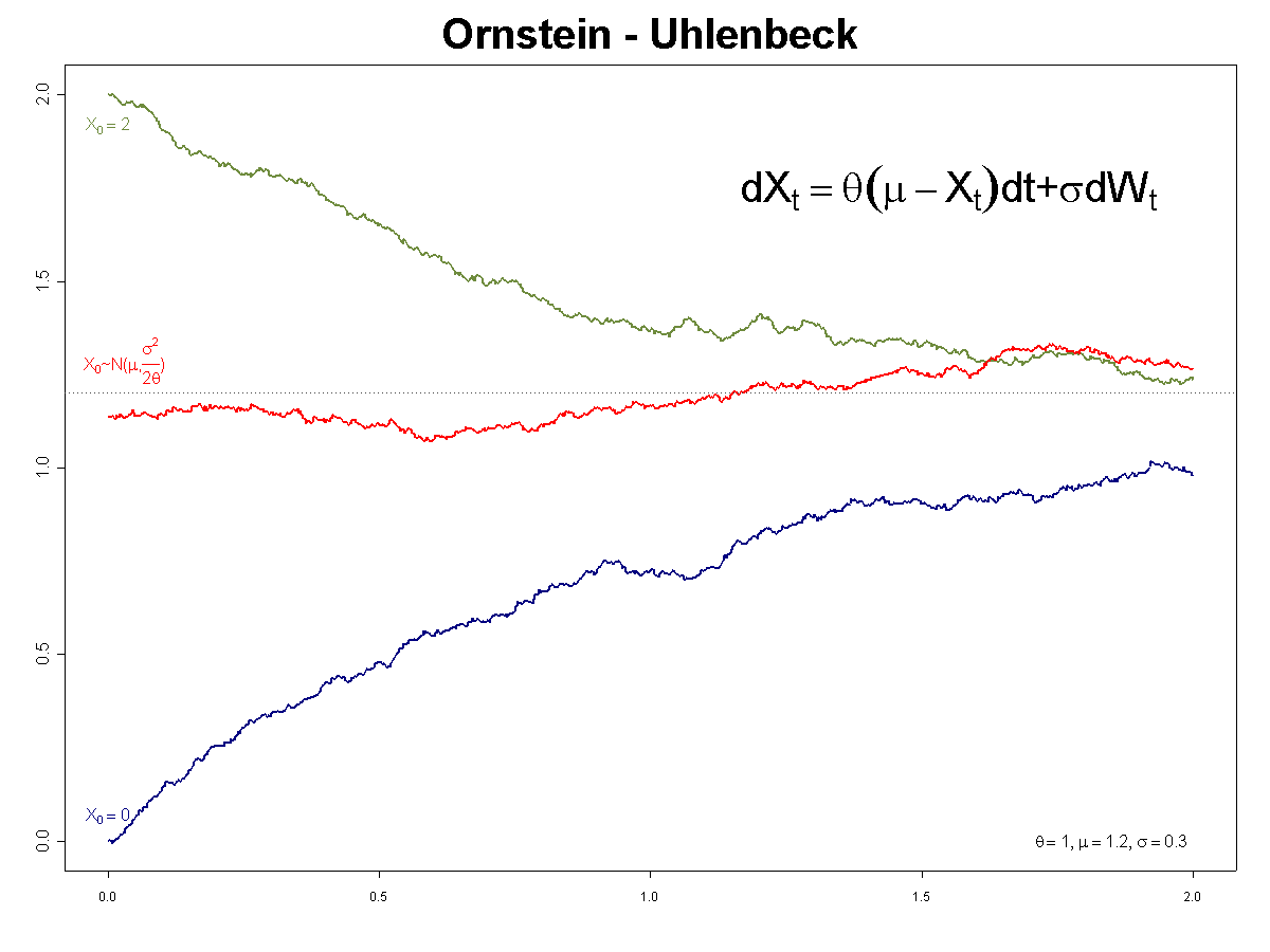
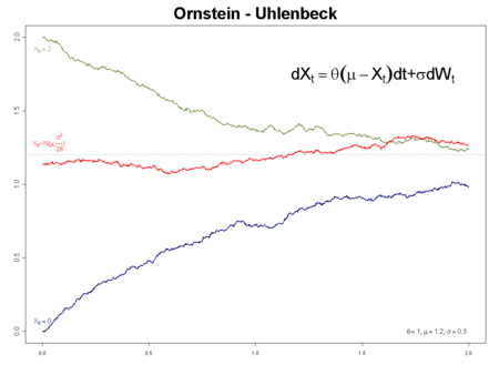three sample paths of different OU-processes with θ = 1, μ = 1.2, σ = 0.3:
blue: initial value a = 0 (a.s.)
green: initial value a = 2 (a.s.)
red: initial value normally distributed so that the process has invariant measure

Solution

This equation is solved^{[clarification needed]} by variation of parameters.^{[citation needed]} Apply Itō–Doeblin's formula to the function

$f(x_t, t) = x_t e^{\theta t} \,$

to get

$\begin{align} df(x_t,t) & = \theta x_t e^{\theta t}\, dt + e^{\theta t}\, dx_t \\ & = e^{\theta t}\theta \mu \, dt + \sigma e^{\theta t}\, dW_t. \end{align}$

Integrating from 0 to t we get

$x_t e^{\theta t} = x_0 + \int_0^t e^{\theta s}\theta \mu \, ds + \int_0^t \sigma e^{\theta s}\, dW_s \,$

whereupon we see

$x_t = x_0 e^{-\theta t} + \mu(1-e^{-\theta t}) + \int_0^t \sigma e^{\theta (s-t)}\, dW_s. \,$

Formulae for moments

From this representation, the first moment is given by (assuming that x₀ is a constant)

$E(x_t)=x_0 e^{-\theta t}+\mu(1-e^{-\theta t}) \!\$

The Itō isometry can be used to calculate the covariance function by

$\begin{align} \operatorname{cov}(x_s,x_t) & = E[(x_s - E[x_s])(x_t - E[x_t])] \\ & = E \left[ \int_0^s \sigma e^{\theta (u-s)}\, dW_u \int_0^t \sigma e^{\theta (v-t)}\, dW_v \right] \\ & = \sigma^2 e^{-\theta (s+t)}E \left[ \int_0^s e^{\theta u}\, dW_u \int_0^t e^{\theta v}\, dW_v \right] \\ & = \frac{\sigma^2}{2\theta} \, e^{-\theta (s+t)}(e^{2\theta \min(s,t)}-1). \end{align}$

Thus if s < t (so that min(s, t) = s), then we have

$\operatorname{cov}(x_s,x_t) = \frac{\sigma^2}{2\theta}\left( e^{-\theta(t-s)} - e^{-\theta(t+s)} \right).$

Alternative representation

It is also possible (and often convenient) to represent x_t (unconditionally, i.e. as $t\rightarrow\infty$) as a scaled time-transformed Wiener process:

$x_t=\mu+{\sigma\over\sqrt{2\theta}}W(e^{2\theta t})e^{-\theta t}$

or conditionally (given x₀) as

$x_t=x_0 e^{-\theta t} +\mu (1-e^{-\theta t})+ {\sigma\over\sqrt{2\theta}}W(e^{2\theta t}-1)e^{-\theta t}.$

The time integral of this process can be used to generate noise with a 1/ƒ power spectrum.

Scaling limit interpretation

The Ornstein–Uhlenbeck process can be interpreted as a scaling limit of a discrete process, in the same way that Brownian motion is a scaling limit of random walks. Consider an urn containing n blue and yellow balls. At each step a ball is chosen at random and replaced by a ball of the opposite colour. Let X_n be the number of blue balls in the urn after n steps. Then $\frac{X_{[nt]} - n/2}{\sqrt{n}}$ converges to a Ornstein–Uhlenbeck process as n tends to infinity.

Fokker–Planck equation representation

The probability density function ƒ(x, t) of the Ornstein–Uhlenbeck process satisfies the Fokker–Planck equation

$\frac{\partial f}{\partial t} = \theta \frac{\partial}{\partial x} [(x - \mu) f] + \frac{\sigma^2}{2} \frac{\partial^2 f}{\partial x^2}$

The general solution of this equation, taking μ = 0 and D = σ² / 2 for simplicity, and the initial condition ξ is,

$f(x,t) = \sqrt{\frac{\theta}{2 \pi D (1-e^{-2\theta t})}} \exp\left\{\frac{-\theta}{2D}\left[\frac{(x - \xi e^{-\theta t})^2}{1-e^{-2\theta t}}\right]\right\}$

The stationary solution of this equation is the limit for time tending to infinity which is a Gaussian distribution with mean μ and variance σ² / (2θ)

$f_s(x) = \sqrt{\frac{\theta}{\pi \sigma^2}}\, e^{-\theta (x-\mu)^2/\sigma^2}.$

Generalizations

It is possible to extend Ornstein–Uhlenbeck processes to processes where the background driving process is a Lévy process.^{[clarification needed]} These processes are widely studied by Ole Barndorff-Nielsen and Neil Shephard,^{[citation needed]} and others.^{[citation needed]}

In addition, in finance, stochastic processes are used the volatility increases for larger values of X. In particular, the CKLS (Chan–Karolyi–Longstaff–Sanders) process^[4] with the volatility term replaced by $\sigma\,x^\gamma\, dW_t$ can be solved in closed form for γ = 1 / 2 or 1, as well as for γ = 0, which corresponds to the conventional OU process.

See also

• The Vasicek model of interest rates is an example of an Ornstein–Uhlenbeck process.
• Short rate model – contains more examples.

Notes

1. ^ ^{a b} Doob 1942
2. ^ Advantages of Pair Trading: Market Neutrality
3. ^ An Ornstein-Uhlenbeck Framework for Pairs Trading
4. ^ Chan et al. (1992)

References

• E. Bibbona, G. Panfilo and P. Tavella: "The Ornstein-Uhlenbeck process as a model of a low pass filtered white noise", Metrologia, 45:S117-S126, 2008. doi:10.1088/0026-1394/45/6/S17
• Chan. K. C., Karolyi, G. A., Longstaff, F. A. & Sanders, A. B.: "An empirical comparison of alternative models of the short-term interest rate", Journal of Finance 52:1209–27, 1992.
• Doob, J.L. (1942), "The Brownian movement and stochastic equations", Annals of Mathematics 43: 351–369 .
• D.T.Gillespie: "Exact numerical simulation of the Ornstein–Uhlenbeck process and its integral", Phys.Rev.E, 54:2084–91, 1996. PMID 9965289 doi:10.1103/PhysRevE.54.2084
• H. Risken: The Fokker–Planck Equation: Method of Solution and Applications, Springer-Verlag, New York, 1989.
• G.E.Uhlenbeck and L.S.Ornstein: "On the theory of Brownian Motion", Phys.Rev., 36:823–841, 1930. doi:10.1103/PhysRev.36.823

External links

• A Stochastic Processes Toolkit for Risk Management, Damiano Brigo, Antonio Dalessandro, Matthias Neugebauer and Fares Triki
• Simulating and Calibrating the Ornstein–Uhlenbeck process^{[dead link]}, M.A. van den Berg
• Calibrating the Ornstein-Uhlenbeck model, M.A. van den Berg
• Maximum likelihood estimation of mean reverting processes, Jose Carlos Garcia Franco