Numerical integration

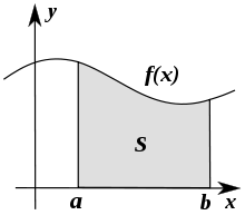Numerical integration consists of finding numerical approximations for the value S

In numerical analysis, numerical integration constitutes a broad family of algorithms for calculating the numerical value of a definite integral, and by extension, the term is also sometimes used to describe the numerical solution of differential equations. This article focuses on calculation of definite integrals. The term numerical quadrature (often abbreviated to quadrature) is more or less a synonym for numerical integration, especially as applied to one-dimensional integrals. Numerical integration over more than one dimension is sometimes described as cubature,^[1] although the meaning of quadrature is understood for higher dimensional integration as well.

The basic problem considered by numerical integration is to compute an approximate solution to a definite integral:

$\int_a^b\! f(x)\, dx.$

If f(x) is a smooth well-behaved function, integrated over a small number of dimensions and the limits of integration are bounded, there are many methods of approximating the integral with arbitrary precision.

Reasons for numerical integration

There are several reasons for carrying out numerical integration. The integrand f(x) may be known only at certain points, such as obtained by sampling. Some embedded systems and other computer applications may need numerical integration for this reason.

A formula for the integrand may be known, but it may be difficult or impossible to find an antiderivative which is an elementary function. An example of such an integrand is f(x) = exp(−x²), the antiderivative of which (the error function, times a constant) cannot be written in elementary form.

It may be possible to find an antiderivative symbolically, but it may be easier to compute a numerical approximation than to compute the antiderivative. That may be the case if the antiderivative is given as an infinite series or product, or if its evaluation requires a special function which is not available.

Methods for one-dimensional integrals

Numerical integration methods can generally be described as combining evaluations of the integrand to get an approximation to the integral. The integrand is evaluated at a finite set of points called integration points and a weighted sum of these values is used to approximate the integral. The integration points and weights depend on the specific method used and the accuracy required from the approximation.

An important part of the analysis of any numerical integration method is to study the behavior of the approximation error as a function of the number of integrand evaluations. A method which yields a small error for a small number of evaluations is usually considered superior. Reducing the number of evaluations of the integrand reduces the number of arithmetic operations involved, and therefore reduces the total round-off error. Also, each evaluation takes time, and the integrand may be arbitrarily complicated.

A 'brute force' kind of numerical integration can be done, if the integrand is reasonably well-behaved (i.e. piecewise continuous and of bounded variation), by evaluating the integrand with very small increments.

Quadrature rules based on interpolating functions

A large class of quadrature rules can be derived by constructing interpolating functions which are easy to integrate. Typically these interpolating functions are polynomials.

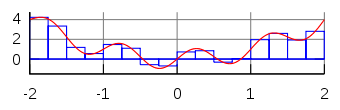Illustration of the rectangle rule.

The simplest method of this type is to let the interpolating function be a constant function (a polynomial of degree zero) which passes through the point ((a+b)/2, f((a+b)/2)). This is called the midpoint rule or rectangle rule.

$\int_a^b f(x)\,dx \approx (b-a) \, f\left(\frac{a+b}{2}\right).$

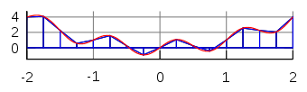Illustration of the trapezoidal rule.

The interpolating function may be an affine function (a polynomial of degree 1) which passes through the points (a, f(a)) and (b, f(b)). This is called the trapezoidal rule.

$\int_a^b f(x)\,dx \approx (b-a) \, \frac{f(a) + f(b)}{2}.$

Illustration of Simpson's rule.

For either one of these rules, we can make a more accurate approximation by breaking up the interval [a, b] into some number n of subintervals, computing an approximation for each subinterval, then adding up all the results. This is called a composite rule, extended rule, or iterated rule. For example, the composite trapezoidal rule can be stated as

$\int_a^b f(x)\,dx \approx \frac{b-a}{n} \left( {f(a) + f(b) \over 2} + \sum_{k=1}^{n-1} f \left( a+k \frac{b-a}{n} \right) \right)$

where the subintervals have the form [k h, (k+1) h], with h = (b−a)/n and k = 0, 1, 2, ..., n−1.

Interpolation with polynomials evaluated at equally spaced points in [a, b] yields the Newton–Cotes formulas, of which the rectangle rule and the trapezoidal rule are examples. Simpson's rule, which is based on a polynomial of order 2, is also a Newton–Cotes formula.

Quadrature rules with equally spaced points have the very convenient property of nesting. The corresponding rule with each interval subdivided includes all the current points, so those integrand values can be re-used.

If we allow the intervals between interpolation points to vary, we find another group of quadrature formulas, such as the Gaussian quadrature formulas. A Gaussian quadrature rule is typically more accurate than a Newton–Cotes rule which requires the same number of function evaluations, if the integrand is smooth (i.e., if it is sufficiently differentiable) Other quadrature methods with varying intervals include Clenshaw–Curtis quadrature (also called Fejér quadrature) methods.

Gaussian quadrature rules do not nest, but the related Gauss–Kronrod quadrature formulas do. Clenshaw–Curtis rules nest.

Adaptive algorithms

For more details on this topic, see Adaptive quadrature.

If f(x) does not have many derivatives at all points, or if the derivatives become large, then Gaussian quadrature is often insufficient. In this case, an algorithm similar to the following will perform better:

def calculate_definite_integral_of_f(f, initial_step_size):
    '''
    This algorithm calculates the definite integral of a function
    from 0 to 1, adaptively, by choosing smaller steps near
    problematic points.
    '''
    x = 0.0
    h = initial_step_size
    accumulator = 0.0
    while x < 1.0:
        if x + h > 1.0:
            h = 1.0 - x
        quad_this_step =
        if error_too_big_in_quadrature_of_over_range(f, [x,x+h]):
            h = make_h_smaller(h)
        else:
            accumulator += quadrature_of_f_over_range(f, [x,x+h])
            x += h
            if error_too_small_in_quadrature_of_over_range(f, [x,x+h]):
                h = make_h_larger(h) # Avoid wasting time on tiny steps.
    return accumulator

Some details of the algorithm require careful thought. For many cases, estimating the error from quadrature over an interval for a function f(x) isn't obvious. One popular solution is to use two different rules of quadrature, and use their difference as an estimate of the error from quadrature. The other problem is deciding what "too large" or "very small" signify. A local criterion for "too large" is that the quadrature error should not be larger than t · h where t, a real number, is the tolerance we wish to set for global error. Then again, if h is already tiny, it may not be worthwhile to make it even smaller even if the quadrature error is apparently large. A global criterion is that the sum of errors on all the intervals should be less than t. This type of error analysis is usually called "a posteriori" since we compute the error after having computed the approximation.

Heuristics for adaptive quadrature are discussed by Forsythe et al. (Section 5.4).

Extrapolation methods

The accuracy of a quadrature rule of the Newton-Cotes type is generally a function of the number of evaluation points. The result is usually more accurate as number of evaluation points increases, or, equivalently, as the width of the step size between the points decreases. It is natural to ask what the result would be if the step size were allowed to approach zero. This can be answered by extrapolating the result from two or more nonzero step sizes, using series acceleration methods such as Richardson extrapolation. The extrapolation function may be a polynomial or rational function. Extrapolation methods are described in more detail by Stoer and Bulirsch (Section 3.4) and are implemented in many of the routines in the QUADPACK library.

Conservative (a priori) error estimation

Let f have a bounded first derivative over [a,b]. The mean value theorem for f, where x < b, gives

$(x - a) f'(y_x) = f(x) - f(a)\,$

for some y_x in [a,x] depending on x. If we integrate in x from a to b on both sides and take the absolute values, we obtain

$\left| \int_a^b f(x)\,dx - (b - a) f(a) \right| = \left| \int_a^b (x - a) f'(y_x)\, dx \right|$

We can further approximate the integral on the right-hand side by bringing the absolute value into the integrand, and replacing the term in f' by an upper bound:

$\left| \int_a^b f(x)\,dx - (b - a) f(a) \right| \leq {(b - a)^2 \over 2} \sup_{a \leq x \leq b} \left| f'(x) \right|$ (**)

(See supremum.) Hence, if we approximate the integral ∫_a^b f(x) dx by the quadrature rule (b − a)f(a) our error is no greater than the right hand side of (**). We can convert this into an error analysis for the Riemann sum (*), giving an upper bound of

${n^{-1} \over 2} \sup_{0 \leq x \leq 1} \left| f'(x) \right|$

for the error term of that particular approximation. (Note that this is precisely the error we calculated for the example f(x) = x.) Using more derivatives, and by tweaking the quadrature, we can do a similar error analysis using a Taylor series (using a partial sum with remainder term) for f. This error analysis gives a strict upper bound on the error, if the derivatives of f are available.

This integration method can be combined with interval arithmetic to produce computer proofs and verified calculations.

Integrals over infinite intervals

Infinite intervals

One way to calculate an integral over infinite interval,

$\int_{-\infty}^{+\infty}f(x) \, dx,$

is to transform it into an integral over a finite interval by any one of several possible changes of variables, for example:

$\int_{-\infty}^{+\infty} f(x) \, dx = \int_{-1}^{+1} f\left( \frac{t}{1-t^2} \right) \frac{1+t^2}{(1-t^2)^2} \, dt,$

The integral over finite interval can then be evaluated by ordinary integration methods.

Half-infinite intervals

An integral over a half-infinite interval can likewise be transformed into an integral over a finite interval by any one of several possible changes of variables, for example:

$\int_a^{+\infty}f(x) \, dx =\int_0^1 f\left(a + \frac{1-t}{t}\right) \frac{dt}{t^2} .$

Similarly,

$\int_{-\infty}^a f(x) \, dx = \int_0^1 f\left(a - \frac{1-t}{t}\right) \frac{dt}{t^2}$

Multidimensional integrals

The quadrature rules discussed so far are all designed to compute one-dimensional integrals. To compute integrals in multiple dimensions, one approach is to phrase the multiple integral as repeated one-dimensional integrals by appealing to Fubini's theorem. This approach requires the function evaluations to grow exponentially as the number of dimensions increases. Two methods are known to overcome this so-called curse of dimensionality.

Monte Carlo

Main article: Monte Carlo integration

Monte Carlo methods and quasi-Monte Carlo methods are easy to apply to multi-dimensional integrals, and may yield greater accuracy for the same number of function evaluations than repeated integrations using one-dimensional methods.

A large class of useful Monte Carlo methods are the so-called Markov chain Monte Carlo algorithms, which include the Metropolis-Hastings algorithm and Gibbs sampling.

Sparse grids

Sparse grids were originally developed by Smolyak for the quadrature of high dimensional functions. The method is always based on a one dimensional quadrature rule, but performs a more sophisticated combination of univariate results.

Connection with differential equations

The problem of evaluating the integral

$\int_a^b f(x)\, dx$

can be reduced to an initial value problem for an ordinary differential equation. If the above integral is denoted by I(b), then the function I satisfies

$I'(x) = f(x), \quad I(a) = 0.$

Methods developed for ordinary differential equations, such as Runge–Kutta methods, can be applied to the restated problem and thus be used to evaluate the integral. For instance, the standard fourth-order Runge–Kutta method applied to the differential equation yields Simpson's rule from above.

The differential equation I ' (x) = ƒ(x) has a special form: the right-hand side contains only the dependent variable (here x) and not the independent variable (here I). This simplifies the theory and algorithms considerably. The problem of evaluating integrals is thus best studied in its own right.

See also

• Numerical ordinary differential equations
• Truncation error (numerical integration)

References

1. ^ Weisstein, Eric W., "Cubature" from MathWorld.

• Philip J. Davis and Philip Rabinowitz, Methods of Numerical Integration.
• George E. Forsythe, Michael A. Malcolm, and Cleve B. Moler. Computer Methods for Mathematical Computations. Englewood Cliffs, NJ: Prentice-Hall, 1977. (See Chapter 5.)
• Press, WH; Teukolsky, SA; Vetterling, WT; Flannery, BP (2007), "Chapter 4. Integration of Functions", Numerical Recipes: The Art of Scientific Computing (3rd ed.), New York: Cambridge University Press, ISBN 978-0-521-88068-8, http://apps.nrbook.com/empanel/index.html?pg=155 
• Josef Stoer and Roland Bulirsch. Introduction to Numerical Analysis. New York: Springer-Verlag, 1980. (See Chapter 3.)

External links

• Integration: Background, Simulations, etc. at Holistic Numerical Methods Institute

Free software for numerical integration

Numerical integration is one of the most intensively studied problems in numerical analysis. Of the many software implementations, we list a few free and open source software packages here:

• QUADPACK (part of SLATEC): description [1], source code [2]. QUADPACK is a collection of algorithms, in Fortran, for numerical integration based on Gaussian quadrature.
• interalg: a solver from OpenOpt/FuncDesigner frameworks, based on interval analysis, guaranteed precision, license: BSD (free for any purposes)
• GSL: The GNU Scientific Library (GSL) is a numerical library written in C which provides a wide range of mathematical routines, like Monte Carlo integration.
• Numerical integration algorithms are found in GAMS class H2.
• ALGLIB is a collection of algorithms, in C# / C++ / Delphi / Visual Basic / etc., for numerical integration (includes Bulirsch-Stoer and Runge-Kutta integrators).
• Cuba is a free-software library of several multi-dimensional integration algorithms.
• Cubature code for adaptive multi-dimensional integration.
• Cubature formulas for the 2D unit disk Derivation, source code for product-type Gaussian cubature with high precision coefficients and nodes.
• High-precision abscissas and weights for Gaussian Quadrature for n = 2, ..., 20, 32, 64, 100, 128, 256, 512, 1024 also contains C language source code under LGPL license.