- Maxwell–Boltzmann statistics
-
Statistical mechanics 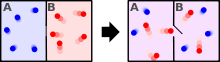
Thermodynamics · Kinetic theory  Distribution of particle speed for 106 oxygen particles at
−100, 20 and 600 degrees Celsius. Speed distribution can be derived from Maxwell–Boltzmann distribution.In statistical mechanics, Maxwell–Boltzmann statistics describes the statistical distribution of material particles over various energy states in thermal equilibrium, when the temperature is high enough and density is low enough to render quantum effects negligible.
The expected number of particles with energy εi for Maxwell–Boltzmann statistics is Ni where:
where:
- Ni is the number of particles in state i
- εi is the energy of the i-th state
- gi is the degeneracy of energy level i, the number of particle's states (excluding the "free particle" state) with energy εi
- μ is the chemical potential
- k is Boltzmann's constant
- T is absolute temperature
- N is the total number of particles
- Z is the partition function
- e(...) is the exponential function
Equivalently, the distribution is sometimes expressed as
where the index i now specifies a particular state rather than the set of all states with energy εi, and

Fermi–Dirac and Bose–Einstein statistics apply when quantum effects are important and the particles are "indistinguishable". Quantum effects appear if the concentration of particles (N/V) ≥ nq. Here nq is the quantum concentration, for which the interparticle distance is equal to the thermal de Broglie wavelength, so that the wavefunctions of the particles are touching but not overlapping. Fermi–Dirac statistics apply to fermions (particles that obey the Pauli exclusion principle), and Bose–Einstein statistics apply to bosons. As the quantum concentration depends on temperature; most systems at high temperatures obey the classical (Maxwell–Boltzmann) limit unless they have a very high density, as for a white dwarf. Both Fermi–Dirac and Bose–Einstein become Maxwell–Boltzmann statistics at high temperature or at low concentration.
Maxwell–Boltzmann statistics are often described as the statistics of "distinguishable" classical particles. In other words the configuration of particle A in state 1 and particle B in state 2 is different from the case where particle B is in state 1 and particle A is in state 2. This assumption leads to the proper (Boltzmann) distribution of particles in the energy states, but yields non-physical results for the entropy, as embodied in the Gibbs paradox. This problem disappears when it is realized that all particles are in fact indistinguishable. Both of these distributions approach the Maxwell–Boltzmann distribution in the limit of high temperature and low density, without the need for any ad hoc assumptions. Maxwell–Boltzmann statistics are particularly useful for studying gases. Fermi–Dirac statistics are most often used for the study of electrons in solids. As such, they form the basis of semiconductor device theory and electronics.
Contents
A derivation of the Maxwell–Boltzmann distribution
Suppose we have a container with a huge number of very small identical particles. Although the particles are identical, we still identify them by drawing numbers on them in the way lottery balls are being labelled with numbers and even colors.
All of those tiny particles are moving inside that container in all directions with great speed. Because the particles are speeding around, they do possess some energy. The Maxwell–Boltzmann distribution is a mathematical function that speaks about how many particles in the container have a certain energy.
It can be so that many particles have the same amount of energy εi. The number of particles with the same energy εi is Ni. The number of particles possessing another energy εj is Nj. In physical speech this statement is lavishly inflated into something complicated which states that those many particles Ni with the same energy amount εi, all occupy a so called "energy level" i . The concept of energy level is used to graphically/mathematically describe and analyse the properties of particles and events experienced by them. Physicists take into consideration the ways particles arrange themself and thus there is more than one way of occupying an energy level and that's the reason why the particles were tagged like lottery ball, to know the intentions of each one of them.
To begin with, let's ignore the degeneracy problem: assume that there is only one single way to put Ni particles into energy level i . What follows next is a bit of combinatorial thinking which has little to do in accurately describing the reservoir of particles.
The number of different ways of performing an ordered selection of one single object from N objects is obviously N. The number of different ways of selecting two objects from N objects, in a particular order, is thus N(N − 1) and that of selecting n objects in a particular order is seen to be N!/(N − n)!. The number of ways of selecting 2 objects from N objects without regard to order is N(N − 1) divided by the number of ways 2 objects can be ordered, which is 2!. It can be seen that the number of ways of selecting n objects from N objects without regard to order is the binomial coefficient: N!/(n!(N − n)!). If we now have a set of boxes labelled a, b, c, d, e, ..., k, then the number of ways of selecting Na objects from a total of N objects and placing them in box a, then selecting Nb objects from the remaining N − Na objects and placing them in box b, then selecting Nc objects from the remaining N − Na − Nb objects and placing them in box c, and continuing until no object is left outside is
and because not even a single object is to be left outside the boxes, implies that the sum made of the terms Na, Nb, Nc, Nd, Ne, ..., Nk must equal N, thus the term (N - Na - Nb - Nc - ... - Nl - Nk)! in the relation above evaluates to 0! which makes possible to write down that relation as
Now going back to the degeneracy problem which characterize the reservoir of particles. If the i-th box has a "degeneracy" of gi, that is, it has gi "sub-boxes", such that any way of filling the i-th box where the number in the sub-boxes is changed is a distinct way of filling the box, then the number of ways of filling the i-th box must be increased by the number of ways of distributing the Ni objects in the gi "sub-boxes". The number of ways of placing Ni distinguishable objects in gi "sub-boxes" is
 . Thus the number of ways W that a total of N particles can be classified into energy levels according to their energies, while each level i having gi distinct states such that the i-th level accommodates Ni particles is:
This is the form for W first derived by Boltzmann. Boltzmann's fundamental equation
 relates the thermodynamic entropy S to the number of microstates W, where k is the Boltzmann constant. It was pointed out by Gibbs however, that the above expression for W does not yield an extensive entropy, and is therefore faulty. This problem is known as the Gibbs paradox The problem is that the particles considered by the above equation are not indistinguishable. In other words, for two particles (A and B) in two energy sublevels the population represented by [A,B] is considered distinct from the population [B,A] while for indistinguishable particles, they are not. If we carry out the argument for indistinguishable particles, we are led to the Bose-Einstein expression for W:
Both the Maxwell-Boltzmann distribution and the Bose-Einstein distribution are only valid for temperatures well above absolute zero, implying that
 . The Maxwell-Boltzmann distribution also requires low density, implying that
  . Under these conditions, we may use Stirling's approximation for the factorial:
to write:
Using the fact that
 for we can again use Stirlings approximation to write:
This is essentially a division by N! of Boltzmann's original expression for W, and this correction is referred to as correct Boltzmann counting.
We wish to find the Ni for which the function W is maximized, while considering the constraint that there is a fixed number of particles
 and a fixed energy
  in the container. The maxima of W and ln(W) are achieved by the same values of Ni and, since it is easier to accomplish mathematically, we will maximize the latter function instead. We constrain our solution using Lagrange multipliers forming the function:
Finally
In order to maximize the expression above we apply Fermat's theorem (stationary points), according to which local extrema, if exist, must be at critical points (partial derivatives vanish):
By solving the equations above (
 ) we arrive to an expression for Ni:
Substituting this expression for Ni into the equation for ln W and assuming that
 yields:
or, differentiating and rearranging:
Boltzmann realized that this is just an expression of the second law of thermodynamics. Identifying dE as the internal energy, the second law of thermodynamics states that for variation only in entropy (S) and particle number (N):
where T is the temperature and μ is the chemical potential. Boltzmann's famous equation
is the realization that the entropy is proportional to ln W with the constant of proportionality being Boltzmann's constant. It follows immediately that β = 1 / kT and α = − μ / kT so that the populations may now be written:Note that the above formula is sometimes written:
where z = exp(μ / kT) is the absolute activity.
Alternatively, we may use the fact that
to obtain the population numbers as
where Z is the partition function defined by:
Another derivation (not as fundamental)
In the above discussion, the Boltzmann distribution function was obtained via directly analysing the multiplicities of a system. Alternatively, one can make use of the canonical ensemble. In a canonical ensemble, a system is in thermal contact with a reservoir. While energy is free to flow between the system and the reservoir, the reservoir is thought to have infinitely large heat capacity as to maintain constant temperature, T, for the combined system.
In the present context, our system is assumed to have the energy levels
 with degeneracies gi. As before, we would like to calculate the probability that our system has energy εi.
If our system is in state
 , then there would be a corresponding number of microstates available to the reservoir. Call this number
  . By assumption, the combined system (of the system we are interested in and the reservoir) is isolated, so all microstates are equally probable. Therefore, for instance, if
  , we can conclude that our system is twice as likely to be in state than
  . In general, if
  is the probability that our system is in state
  ,
,Since the entropy of the reservoir
 , the above becomes
Next we recall the thermodynamic identity (from the first law of thermodynamics):
In a canonical ensemble, there is no exchange of particles, so the dNR term is zero. Similarly, dVR = 0. This gives
where
 and
and  denote the energies of the reservoir and the system at si, respectively. For the second equality we have used the conservation of energy. Substituting into the first equation relating
  :
:which implies, for any state s of the system
where Z is an appropriately chosen "constant" to make total probability 1. (Z is constant provided that the temperature T is invariant.) It is obvious that
where the index s runs through all microstates of the system. Z is sometimes called the Boltzmann sum over states (or "Zustandsumme" in the original German). If we index the summation via the energy eigenvalues instead of all possible states, degeneracy must be taken into account. The probability of our system having energy
is simply the sum of the probabilities of all corresponding microstates:where, with obvious modification,
this is the same result as before.
Comments
- Notice that in this formulation, the initial assumption "... suppose the system has total N particles..." is dispensed with. Indeed, the number of particles possessed by the system plays no role in arriving at the distribution. Rather, how many particles would occupy states with energy follows as an easy consequence.
- What has been presented above is essentially a derivation of the canonical partition function. As one can tell by comparing the definitions, the Boltzmann sum over states is really no different from the canonical partition function.
- Exactly the same approach can be used to derive Fermi–Dirac and Bose–Einstein statistics. However, there one would replace the canonical ensemble with the grand canonical ensemble, since there is exchange of particles between the system and the reservoir. Also, the system one considers in those cases is a single particle state, not a particle. (In the above discussion, we could have assumed our system to be a single atom.)
Limits of applicability
The Bose–Einstein and Fermi–Dirac distributions may be written:
Assuming the minimum value of εi is small, it can be seen that the condition under which the Maxwell–Boltzmann distribution is valid is when
For an ideal gas, we can calculate the chemical potential using the development in the Sackur–Tetrode article to show that:
where E is the total internal energy, S is the entropy, V is the volume, and Λ is the thermal de Broglie wavelength. The condition for the applicability of the Maxwell–Boltzmann distribution for an ideal gas is again shown to be
See also
References
Bibliography
- Carter, Ashley H., "Classical and Statistical Thermodynamics", Prentice–Hall, Inc., 2001, New Jersey.
- Raj Pathria, "Statistical Mechanics", Butterworth–Heinemann, 1996.
Statistical mechanics Statistical ensembles Statistical thermodynamics Partition functions Translational • Vibrational • RotationalEquations of state Entropy Particle statistics Maxwell–Boltzmann statistics • Fermi–Dirac statistics • Bose–Einstein statisticsStatistical field theory Conformal field theory • Osterwalder–Schrader axiomsSee also Categories:- Fundamental physics concepts
- Maxwell–Boltzmann statistics


![\ln W=\ln\left[\prod\limits_{i=1}^{n}\frac{g_i^{N_i}}{N_i!}\right] \approx \sum\limits_{i=1}^n\left(N_i\ln g_i-N_i\ln N_i + N_i\right)](7/85722d857301bca8c60b3b902c083190.png)


Wikimedia Foundation. 2010.