- Coherent states
-
In quantum mechanics a coherent state is a specific kind of quantum state of the quantum harmonic oscillator whose dynamics most closely resembles the oscillating behaviour of a classical harmonic oscillator. It was the first example of quantum dynamics when Erwin Schrödinger derived it in 1926 while searching for solutions of the Schrödinger equation that satisfy the correspondence principle. [1] The quantum harmonic oscillator and hence, the coherent states, arises in the quantum theory of a wide range of physical systems [2] For instance, a coherent state describes the oscillating motion of the particle in a quadratic potential well (for an early reference, see e.g. Schiff's textbook [3]). These states, defined as eigenvectors of the lowering operator and forming an overcomplete family, were introduced in the early papers of John R. Klauder, e.g. [4]. In the quantum theory of light (quantum electrodynamics) and other bosonic quantum field theories, coherent states were introduced by the work of Roy J. Glauber in 1963. Here the coherent state of a field describes an oscillating field, the closest quantum state to a classical sinusoidal wave such as a continuous laser wave.
However, the concept of coherent states has been considerably generalized, to the extent that it has become a major topic in mathematical physics and in applied mathematics, with applications ranging from quantization to signal processing and image processing (see Coherent states in mathematical physics). For that reason, the coherent states associated to the quantum harmonic oscillator are usually called canonical coherent states (CCS) or standard coherent states or Gaussian states in the literature.
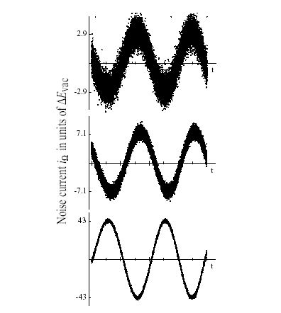
 Figure 1: The electric field, measured by optical homodyne detection, as a function of phase for three coherent states emitted by a Nd:YAG laser. The amount of quantum noise in the electric field is completely independent of the phase. As the field strength, i.e. the oscillation amplitude α of the coherent state is increased, the quantum noise or uncertainty is constant at 1/2, and so becomes less and less significant. In the limit of large field the state becomes a good approximation of a noiseless stable classical wave. The average photon numbers of the three states from top to bottom are <n>=4.2, 25.2, 924.5 (source:,[5] external link 1)
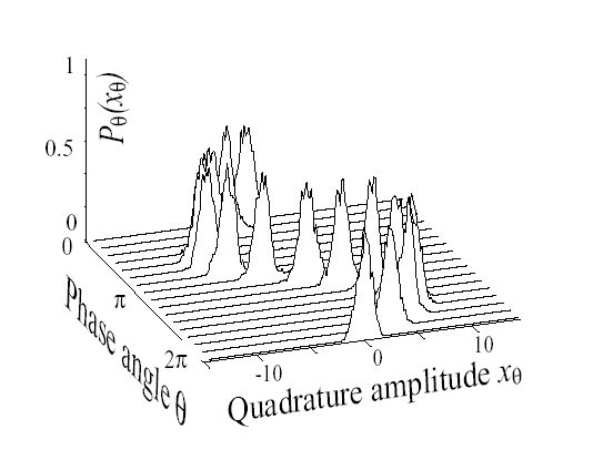
 Figure 2: The oscillating wave packet corresponding to the second coherent state depicted in Figure 1. At each phase of the light field, the distribution is a Gaussian of constant width.
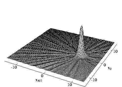
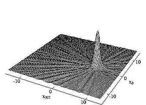 Figure 3: Wigner function of the coherent state depicted in Figure 2. The distribution is centered on state's amplitude α and is symmetric around this point. The ripples are due to experimental errors.
Coherent states in quantum optics
In quantum mechanics a coherent state is a specific kind of quantum state, applicable to the quantum harmonic oscillator, the electromagnetic field, etc. [2] [6] [7]that describes a maximal kind of coherence and a classical kind of behavior. Erwin Schrödinger derived it as a minimum uncertainty Gaussian wavepacket in 1926 while searching for solutions of the Schrödinger equation that satisfy the correspondence principle [1]. It is a minimum uncertainty state, with the single free parameter chosen to make the relative dispersion (standard deviation divided by the mean) equal for position and momentum, each being equally small at high energy. Further, contrary to the energy eigenstates of the system, the time evolution of a coherent state is concentrated along the classical trajectories. The quantum linear harmonic oscillator and hence, the coherent states, arise in the quantum theory of a wide range of physical systems. They are found in the quantum theory of light (quantum electrodynamics) and other bosonic quantum field theories.
While minimum uncertainty Gaussian wave-packets were well-known, they did not attract much attention until Roy J. Glauber, in 1963, provided a complete quantum-theoretic description of coherence in the electromagnetic field.[8] In this respect, the concurrent contribution of E.C.G. Sudarshan should not be omitted, [9] (there is, however, a note in Glauber's paper that reads: "Uses of these states as generating functions for the n-quantum states have, however, been made by J. Schwinger [10]). Glauber was prompted to do this to provide a description of the Hanbury-Brown & Twiss experiment that generated very wide baseline (hundreds or thousands of miles) interference patterns that could be used to determine stellar diameters. This opened the door to a much more comprehensive understanding of coherence. (For more, see Quantum mechanical description.)
In classical optics light is thought of as electromagnetic waves radiating from a source. Often, coherent laser light is thought of as light that is emitted by many such sources that are in phase. Actually, the picture of one photon being in-phase with another is not valid in quantum theory. Laser radiation is produced in a resonant cavity where the resonant frequency of the cavity is the same as the frequency associated with the atomic transitions providing energy flow into the field. As energy in the resonant mode builds up, the probability for stimulated emission, in that mode only, increases. That is a positive feedback loop in which the amplitude in the resonant mode increases exponentially until some non-linear effects limit it. As a counter-example, a light bulb radiates light into a continuum of modes, and there is nothing that selects any one mode over the other. The emission process is highly random in space and time (see thermal light). In a laser, however, light is emitted into a resonant mode, and that mode is highly coherent. Thus, laser light is idealized as a coherent state. (Classically we describe such a state by an electric field oscillating as a stable wave. See Fig.1)
The energy eigenstates of the linear harmonic oscillator (e.g., masses on springs, lattice vibrations in a solid, vibrational motions of nuclei in molecules, or oscillations in the electromagnetic field) are fixed-number quantum states. The Fock state (e.g. a single photon) is the most particle-like state; it has a fixed number of particles, and phase is indeterminate. A coherent state distributes its quantum-mechanical uncertainty equally between the canonically conjugate coordinates, position and momentum, and the relative uncertainty in phase [defined heuristically] and amplitude are roughly equal—and small at high amplitude.
Quantum mechanical definition
Mathematically, the coherent state
 is defined to be the right eigenstate of the annihilation operator
  . Formally, this reads:
Since
is not hermitian, α is a complex number that is not necessarily real, and can be represented aswhere
 is a real number. Here
  and are called the amplitude and phase of the state, respectively. The state
  is called a canonical coherent state in the literature, since there are many other types of coherent states, as can be seen in the companion article Coherent states in mathematical physics.
Physically, this formula means that a coherent state is left unchanged by the detection (or annihilation) of field excitation or, say, a particle. The eigenstate of the annihilation operator has a Poissonian number distribution (as shown below). A Poisson distribution is a necessary and sufficient condition that all detections are statistically independent. Compare this to a single-particle state (
 Fock state): once one particle is detected, there is zero probability of detecting another.
The derivation of this will make use of dimensionless operators,
 and
and  , usually called field quadratures in quantum optics. These operators are related to the position and momentum of a mass
  on a spring with constant
  :
:
For an optical field,
 and
and 
are the real and imaginary components of the mode of the electric field.
With these (dimensionless!) operators, the Hamiltonian of either system becomes
![{H}=\hbar \omega \left({P}^{2}+{X}^{2} \right)\text{,}
\qquad\text{with}\qquad
\left[ {X},{P} \right]\equiv {XP}-{PX}=\frac{i}{2}\,{I}.](4/dc470bc89f69aff969144fa7c47f7d76.png)
Erwin Schrödinger was searching for the most classical-like states when he first introduced minimum uncertainty Gaussian wave-packets. The quantum state of the harmonic oscillator that minimizes the uncertainty relation with uncertainty equally distributed between
and satisfies the equation .
.It is an eigenstate of the operator (X + iP). (If the uncertainty is not balanced between
and , the state is now called a squeezed coherent state.)Schrödinger found minimum uncertainty states for the linear harmonic oscillator to be the eigenstates of
 , and using the notation for multi-photon states, Glauber found the state of complete coherence to all orders in the electromagnetic field to be the right eigenstate of the annihilation operator—formally, in a mathematical sense, the same state. The name coherent state took hold after Glauber's work.
The coherent state's location in the complex plane (phase space) is centered at the position and momentum of a classical oscillator of the same phase
and amplitude (or the same complex electric field value for an electromagnetic wave). As shown in Figure 5, the uncertainty, equally spread in all directions, is represented by a disk with diameter 1/2. As the phase increases the coherent state circles the origin and the disk neither distorts nor spreads. This is the most similar a quantum state can be to a single point in phase space.Since the uncertainty (and hence measurement noise) stays constant at 1/2 as the amplitude of the oscillation increases, the state behaves more and more like a sinusoidal wave, as shown in Figure 1. And, since the vacuum state
 is just the coherent state with α = 0, all coherent states have the same uncertainty as the vacuum. Therefore one can interpret the quantum noise of a coherent state as being due to the vacuum fluctuations.
The notation
does not refer to a Fock state. For example, at α = 1, one should not mistake  as a single-photon Fock state—it represents a Poisson distribution of fixed number states with a mean photon number of unity.
The formal solution of the eigenvalue equation is the vacuum state displaced to a location α in phase space, i.e., it is obtained by letting the unitary displacement operator D(α) operate on the vacuum:
 ,
,
where
 and
and  . This can be easily seen, as can virtually all results involving coherent states, using the representation of the coherent state in the basis of Fock states:
 .
.
where
 are energy (number) eigenvectors of the Hamiltonian
  . For the corresponding Poissonian distribution, the probability of detecting
  photons is:
Similarly, the average photon number in a coherent state is
 and the variance is
  .
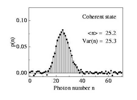
.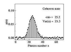 Figure 4: The probability of detecting n photons, the photon number distribution, of the coherent state in Figure 3. As is necessary for a Poissonian distribution the mean photon number is equal to the variance of the photon number distribution. Bars refer to theory, dots to experimental values.
 Figure 5: Phase space plot of a coherent state. This shows that the uncertainty in a coherent state is equally distributed in all directions. The horizontal and vertical axes are the X and P quadratures of the field, respectively (see text). The red dots on the x-axis trace out the boundaries of the quantum noise in Figure 1.
In the limit of large α these detection statistics are equivalent to that of a classical stable wave for all (large) values of
 . These results apply to detection results at a single detector and thus relate to first order coherence (see degree of coherence). However, for measurements correlating detections at multiple detectors, higher-order coherence is involved (e.g., intensity correlations, second order coherence, at two detectors). Glauber's definition of quantum coherence involves nth-order correlation functions (n-th order coherence) for all n. The perfect coherent state has all n-orders of correlation equal to 1 (coherent). It is perfectly coherent to all orders.
Roy J. Glauber's work was prompted by the results of Hanbury-Brown and Twiss that produced long-range (hundreds or thousands of miles) first-order interference patterns through the use of intensity fluctuations (lack of second order coherence), with narrow band filters (partial first order coherence) at each detector. (One can imagine, over very short durations, a near-instantaneous interference pattern from the two detectors, due to the narrow band filters, that dances around randomly due to the shifting relative phase difference. With a coincidence counter, the dancing interference pattern would be stronger at times of increased intensity [common to both beams], and that pattern would be stronger than the background noise.) Almost all of optics had been concerned with first order coherence. The Hanbury-Brown and Twiss results prompted Glauber to look at higher order coherence, and he came up with a complete quantum-theoretic description of coherence to all orders in the electromagnetic field (and a quantum-theoretic description of signal-plus-noise). He coined the term coherent state and showed that they are produced when a classical electrical current interacts with the electromagnetic field.
At
 , from Figure 5, simple geometry gives
  . From this we can see that there is a tradeoff between number uncertainty and phase uncertainty
  , which sometimes can be interpreted as the number-phase uncertainty relation. This is not a formal uncertainty relation: there is no uniquely defined phase operator in quantum mechanics [11] [12] [13] [14] [15] [16] [17] [18]
The wavefunction of a coherent state
To find the wavefunction of the coherent state, it is easiest to employ the Heisenberg picture of the quantum harmonic oscillator for the coherent state
 . Now we have that
So the coherent state is an eigenstate of the annihilation operator in the Heisenberg picture. It is easy to show that in the Schrödinger picture the same eigenvalue
 occurs:
 .
.
Taking the coordinate representations we obtain the following differential equation
which is easily solved to give
where
 is a still undetermined phase, which we must fix by demanding that the wavefunction satisfies the Schrödinger equation. We obtain that
where
 is the initial phase of the eigenvalue, i.e.
  . The mean position and momentum of the wavepacket ψ(α) are
Mathematical characteristics of the canonical coherent states
The canonical coherent states described so far have three properties that are mutually equivalent, since each of them completely specifies the state
, namely,- They are eigenvectors of the annihilation operator:
 .
. - They are obtained from the vacuum by application of a unitary displacement operator:
 .
. - They are states of (balanced) minimal uncertainty:
 .
.
Each of these properties may lead to generalizations, in general different from each other (see the article 'Coherent states in mathematical physics' for some of these). We emphasize that coherent states have mathematical features that are very different from those of a Fock state; for instance two different coherent states are not orthogonal:
(this is related to the fact that they are eigenvectors of the non-self-adjoint operator
).Thus, if the oscillator is in the quantum state
it is also with nonzero probability in the other quantum state  (but the farther apart the states are situated in phase space, the lower the probability is). However, since they obey a closure relation, any state can be decomposed on the set of coherent states. They hence form an overcomplete basis in which one can diagonally decompose any state. This is the premise for the Sudarshan-Glauber P representation. This closure relation can be expressed by the resolution of the identity operator I in the vector space of quantum states:
 .
.
Another difficulty is that
 has no eigenket (and has no eigenbra). The following formal equality is the closest substitute and turns out to be very useful for technical computations:
The last state is known as Agarwal state or photon-added coherent state and denoted as
 Normalized Agarwal states for order n can be expressed as
 ![|\alpha,n\rangle=[{\hat{a}^{\dagger}]}^n|\alpha\rangle / \| [{\hat{a}^{\dagger}]}^n|\alpha\rangle \|](6/846b2c9132226517526da9da1961b83a.png)
The resolution of the identity may be derived (restricting to one spatial dimension for simplicity) by taking matrix elements between eigenstates of position,
 , on both sides of the equation. On the right-hand side, this immediately gives δ(x − y). On the left-hand side, the same is obtained by inserting
from the previous section (time is arbitrary), then integrating over
 using the Fourier representation of the delta function, and then performing a Gaussian integral over
  .
.The resolution of the identity may also be expressed in terms of particle position and momentum. For each coordinate dimension, using an adapted notation with new meaning of x,
the closure relation of coherent states reads
This can be inserted in any quantum-mechanical expectation value, relating it to some quasi-classical phase-space integral and explaining, in particular, the origin of normalisation factors
 for classical partition functions consistent with quantum mechanics.
In addition to being an exact eigenstate of annihilation operators, a coherent state is an approximate common eigenstate of particle position and momentum. Restricting to one dimension again,
The error in these approximations is measured by the uncertainties of position and momentum,
Coherent states of Bose–Einstein condensates
- A Bose–Einstein condensate (BEC) is a collection of boson atoms that are all in the same quantum state. In a thermodynamic system, the ground state becomes macroscopically occupied below a critical temperature — roughly when the thermal de Broglie wavelength is longer than the interatomic spacing. Superfluidity in liquid Helium-4 is believed to be associated with the Bose–Einstein condensation in an ideal gas. But 4He has strong interactions, and the liquid structure factor (a 2nd-order statistic) plays an important role. The use of a coherent state to represent the superfluid component of 4He provided a good estimate of the condensate / non-condensate fractions in superfluidity,consistent with results of slow neutron scattering. [19] [20] [21] Most of the special superfluid properties follow directly from the use of a coherent state to represent the superfluid component — that acts as a macroscopically occupied single-body state with well-defined amplitude and phase over the entire volume. (The superfluid component of 4He goes from zero at the transition temperature to 100% at absolute zero. But the condensate fraction is about 6%[22] at absolute zero temperature, T=0° K.)
- Early in the study of superfluidity, Penrose and Onsager proposed a metric ("order parameter") for superfluidity.[23] It was represented by a macroscopic factored component (a macroscopic eigenvalue) in the first-order reduced density matrix. Later, C. N. Yang [24] proposed a more generalized measure of macroscopic quantum coherence, called "Off-Diagonal Long-Range Order" (ODLRO), that included fermion as well as boson systems. ODLRO exists whenever there is a macroscopically large factored component (eigenvalue) in a reduced density matrix of any order. Superfluidity corresponds to a large factored component in the first-order reduced density matrix. (And, all higher order reduced density matrices behaved similarly.) Superconductivity involves a large factored component in the 2nd-order ("Cooper electron-pair") reduced density matrix.
- The orders of reduced density matrices used to describe macroscopic quantum coherence in superfluids are formally the same as the correlation functions used to describe orders of coherence in radiation. Both are examples of macroscopic quantum coherence. The macroscopically large coherent component, plus noise, in the electromagnetic field, as given by Glauber's description of signal-plus-noise, is formally the same as the macroscopically large superfluid component plus normal fluid component in the two-fluid model of superfluidity.
- Every-day electromagnetic radiation, such as radio and TV waves, is also an example of near coherent states (macroscopic quantum coherence). That should "give one pause" regarding the conventional demarcation between quantum and classical.
Coherent electron states in superconductivity
- Electrons are fermions, but when they pair up into Cooper pairs they act as bosons, and so can collectively form a coherent state at low temperatures. Such coherent states are part of the explanation of effects such as the Quantum Hall effect in low-temperature superconducting semiconductors.
Generalizations
- According to Gilmore and Perelomov, who showed it independently, the construction of coherent states may be seen as a problem in group theory, and thus coherent states may be associated to groups different from the Heisenberg group, which leads to the canonical coherent states discussed above.[25][26][27][28] Moreover, these coherent states may be generalized to quantum groups. These topics, with references to original work, are discussed in detail in Coherent states in mathematical physics.
- In quantum field theory and string theory, a generalization of coherent states to the case of infinitely many degrees of freedom is used to define a vacuum state with a different vacuum expectation value from the original vacuum.
- In one-dimensional many-body quantum systems with fermionic degrees of freedom, low energy excited states can be approximated as coherent states of a bosonic field operator that creates particle-hole excitations. This approach is called bosonization.
- The Gaussian coherent states of nonrelativistic quantum mechanics can be generalized to relativistic coherent states of Klein-Gordon and Dirac particles. [29] [30]
- Coherent states have also appeared in works on loop quantum gravity or for the construction of (semi)classical canonical quantum general relativity. See, for instance, [31][32].
See also
- Coherent states in mathematical physics
- Quantum field theory
- Quantum optics
- Electromagnetic field
- degree of coherence
- quantum amplifier
External links
- Quantum states of the light field
- Glauber States: Coherent states of Quantum Harmonic Oscillator
- Measure a coherent state with photon statistics interactive
References
- ^ a b E. Schrödinger, Der stetige Übergang von der Mikro- zur Makromechanik, Naturwissenschaften 14 (1926) 664-666.
- ^ a b J.R. Klauder and B. Skagerstam, Coherent States, World Scientific, Singapore, 1985.
- ^ I.I. Schiff, Quantum Mechanics, McGraw Hill, New York, 1955.
- ^ J. R. Klauder, The action option and a Feynman quantization of spinor fields in terms of ordinary c-numbers, Ann. Physics 11 (1960) 123–168.
- ^ G. Breitenbach, S. Schiller, and J. Mlynek, Measurement of the quantum states of squeezed light, Nature 387 (1997) 471-475
- ^ W-M. Zhang, D. H. Feng, and R. Gilmore, Coherent states: Theory and some applications, Rev. Mod. Phys. 62 (1990) 867-927.
- ^ J-P. Gazeau, Coherent States in Quantum Physics, Wiley-VCH, Berlin, 2009.
- ^ R.J. Glauber, Coherent and incoherent states of radiation field,Phys. Rev. 131 (1963) 2766-2788.
- ^ E.C.G. Sudarshan, Equivalence of semiclassical and quantum mechanical descriptions of statistical light beams, Phys. Rev. Lett. 10 (1963) 277-279.
- ^ J. Schwinger, Theory of quantized fields. III, Phys. Rev. 91 (1953) 728-740
- ^ L. Susskind and J. Glogower, Quantum mechanical phase and time operator,Physics 1 (1963) 49.
- ^ P. Carruthers and M.N. Nieto, Phase and angle variables in quantum mechanics,Rev. Mod. Phys. 40 (1968) 411-440.
- ^ S.M. Barnett and D.T. Pegg, On the Hermitian optical phase operator,J. Mod. Opt. 36 (1989) 7-19.
- ^ P. Busch, M. Grabowski and P.J. Lahti, Who is afraid of POV measures? Unified approach to quantum phase observables, Ann. Phys. (N.Y.) 237 (1995) 1-11.
- ^ V.V. Dodonov, 'Nonclassical' states in quantum optics: a 'squeezed' review of the first 75 years, J. Opt. B: Quantum Semiclass. Opt. 4 (2002) R1-R33.
- ^ V.V. Dodonov and V.I.Man'ko (eds), Theory of Nonclassical States of Light, Taylor \& Francis, London, New York, 2003.
- ^ A. Vourdas, Analytic representations in quantum mechanics, J. Phys. A: Math. Gen. 39 (2006) R65-R141.
- ^ J-P. Gazeau,Coherent States in Quantum Physics, Wiley-VCH, Berlin, 2009.
- ^ G. J. Hyland, G. Rowlands, and F. W. Cummings, A proposal for an experimental determination of the equilibrium condensate fraction in superfluid helium, Phys. Lett. 31A (1970) 465-466.
- ^ J. Mayers, The Bose–Einstein condensation, phase coherence, and two-fluid behavior in He-4, Phys. Rev. Lett. 92 (2004) 135302.
- ^ J. Mayers, The Bose–Einstein condensation and two-fluid behavior in He-4, Phys. Rev. B 74 (2006) 014516.
- ^ A.C. Olinto, Condensate fraction in superfluid He-4, Phys. Rev. B 35 (1986) 4771-4774.
- ^ O. Penrose and L. Onsager, Bose–Einstein condensation and liquid Helium, Phys. Rev. 104(1956) 576-584.
- ^ C. N. Yang, Concept of Off-Diagonal Long-Range Order and the quantum phases of liquid He and superconductors, Rev. Mod Phys. 34 (1962) 694-704.
- ^ A. M. Perelomov, Coherent states for arbitrary Lie groups, Commun. Math. Phys. 26 (1972) 222-236; arXiv: math-ph/0203002.
- ^ A. Perelomov, Generalized coherent states and their applications, Springer, Berlin 1986.
- ^ R. Gilmore, Geometry of symmetrized states, Ann. Phys. (NY) 74 (1972) 391-463.
- ^ R. Gilmore, On properties of coherent states, Rev. Mex. Fis. 23 (1974) 143-187.
- ^ G. Kaiser, Quantum Physics, Relativity, and Complex Spacetime: Towards a New Synthesis, North-Holland, Amsterdam, 1990.
- ^ S.T. Ali, J-P. Antoine, and J-P. Gazeau, Coherent States, Wavelets and Their Generalizations, Springer-Verlag, New York, Berlin, Heidelberg, 2000.
- ^ A. Ashtekar, J. Lewandowski, D. Marolf, J. Mourão and T. Thiemann, Coherent state transforms for spaces of connections, J. Funct. Anal. 135 (1996) 519-551.
- ^ H. Sahlmann, T. Thiemann and O. Winkler, Coherent states for canonical quantum general relativity and the infinite tensor product extension, Nucl. Phys. B 606 (2001) 401-440.
Categories:


![~\psi^{(\alpha)}(x,t)=\left(\frac{m\omega}{\pi\hbar}\right)^{1/4}e^{-\frac{m\omega}{2\hbar}\left(x-\sqrt{\frac{2\hbar}{m\omega}}\Re[\alpha(t)]\right)^2+i\sqrt{\frac{2m\omega}{\hbar}}\Im[\alpha(t)]x+i\delta(t)}\;,](3/b537c7b4565060eb5e12f09eb704b53b.png)

![\langle \hat{x}(t) \rangle = \sqrt{\frac{2\hbar}{m\omega}}\Re[\alpha(t)] \qquad \qquad
\langle \hat{p}(t) \rangle = \sqrt{2m\hbar\omega}\Im[\alpha(t)]](3/b536f88fdc3426b69cdeb66c69e3076b.png)


Wikimedia Foundation. 2010.