- Connected-component labeling
-
Connected-component labeling (alternatively connected-component analysis, blob extraction, region labeling, blob discovery, or region extraction) is an algorithmic application of graph theory, where subsets of connected components are uniquely labeled based on a given heuristic. Connected-component labeling is not to be confused with segmentation.
Connected-component labeling is used in computer vision to detect connected regions in binary digital images, although color images and data with higher-dimensionality can also be processed.[1][2] When integrated into an image recognition system or human-computer interaction interface, connected component labeling can operate on a variety of information.[3][4] Blob extraction is generally performed on the resulting binary image from a thresholding step. Blobs may be counted, filtered, and tracked.
Blob extraction is related to but distinct from blob detection.
Contents
Overview
 4-connectivity
 8-connectivity
A graph, containing vertices and connecting edges, is constructed from relevant input data. The vertices contain information required by the comparison heuristic, while the edges indicate connected 'neighbors'. An algorithm traverses the graph, labeling the vertices based on the connectivity and relative values of their neighbors. Connectivity is determined by the medium; image graphs, for example, can be 4-connected or 8-connected.[5]
Following the labeling stage, the graph may be partitioned into subsets, after which the original information can be recovered and processed .
Algorithms
The algorithms discussed can be generalized to arbitrary dimensions, albeit with increased time and space complexity.
Two-pass
Relatively simple to implement and understand, the two-pass algorithm[6] iterates through 2-dimensional, binary data. The algorithm makes two passes over the image: one pass to record equivalences and assign temporary labels and the second to replace each temporary label by the label of its equivalence class.
The input data can be modified in situ (which carries the risk of data corruption), or labeling information can be maintained in an additional data structure.
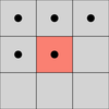
Connectivity checks are carried out by checking the labels of pixels that are North-East, North, North-West and West of the current pixel (assuming 8-connectivity). 4-connectivity uses only North and West neighbors of the current pixel. The following conditions are checked to determine the value of the label to be assigned to the current pixel (4-connectivity is assumed)
Conditions to check:
- Does the pixel to the left (West) have the same value?
- Yes - We are in the same region. Assign the same label to the current pixel
- No - Check next condition
- Do the pixels to the North and West of the current pixel have the same value but not the same label?
- Yes - We know that the North and West pixels belong to the same region and must be merged. Assign the current pixel the minimum of the North and West labels, and record their equivalence relationship
- No - Check next condition
- Does the pixel to the left (West) have a different value and the one to the North the same value?
- Yes - Assign the label of the North pixel to the current pixel
- No - Check next condition
- Do the pixel's North and West neighbors have different pixel values?
- Yes - Create a new label id and assign it to the current pixel
The algorithm continues this way, and creates new region labels whenever necessary. The key to a fast algorithm, however, is how this merging is done. This algorithm uses the union-find data structure which provides excellent performance for keeping track of equivalence relationships.[7] Union-find essentially stores labels which correspond to the same blob in a disjoint-set data structure, making it easy to remember the equivalence of two labels by the use of an interface method E.g.: findSet(l). findSet(l) returns the minimum label value that is equivalent to the function argument 'l'.
Once the initial labeling and equivalence recording is completed, the second pass merely replaces each pixel label with the it's equivalent disjoint-set representative element.
A raster-scanning algorithm for connected-region extraction is presented below.
On the first pass:
- Iterate through each element of the data by column, then by row (Raster Scanning)
- If the element is not the background
- Get the neighboring elements of the current element
- If there are no neighbors, uniquely label the current element and continue
- Otherwise, find the neighbor with the smallest label and assign it to the current element
- Store the equivalence between neighboring labels
On the second pass:
- Iterate through each element of the data by column, then by row
- If the element is not the background
- Relabel the element with the lowest equivalent label
Here, the background is a classification, specific to the data, used to distinguish salient elements from the foreground. If the background variable is omitted, then the two-pass algorithm will treat the background as another region.
Graphical example of two-pass algorithm
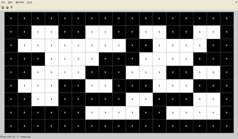
1. The array from which connected regions are to be extracted is given below
2. After the first pass, the following labels are generated. Note that a total of 7 labels are generated in accordance with the conditions highlighted above.
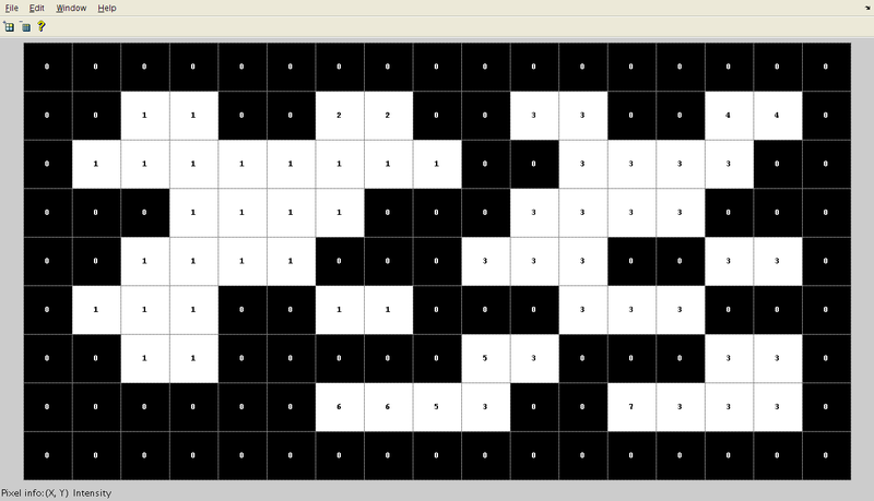
The label equivalence relationships generated are,
Set ID Equivalent Labels 1 1,2 2 1,2 3 3,4,5,6,7 4 3,4,5,6,7 5 3,4,5,6,7 6 3,4,5,6,7 7 3,4,5,6,7 3. Array generated after the merging of labels is carried out. Here, the label value that was the smallest for a given region "floods" throughout the connected region and gives two distinct labels, and hence two distinct labels.
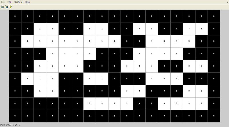
4. Final result in color to clearly see two different regions that have been found in the array.
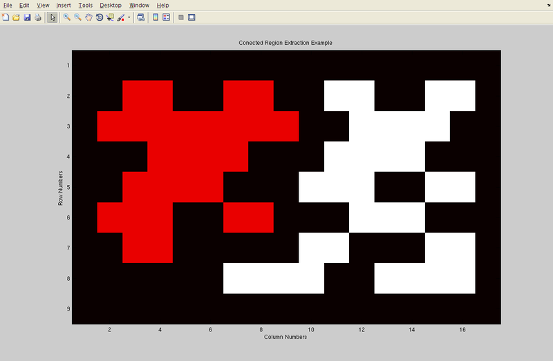
 Sample graphical output from running the two-pass algorithm on a binary image. The first image is unprocessed, while the last one has been recolored with label information. Darker hues indicate the neighbors of the pixel being processed.
The pseudocode is as follows:
algorithm TwoPass(data)
   linked = []
   labels = structure with dimensions of data, initialized with the value of Background

   First pass

   for row in data:
       for column in row:
           if data[row][column] is not Background

               neighbors = connected elements with the current element's label

               if neighbors is empty
                   linked[NextLabel] = set containing NextLabel
                   labels[row][column] = NextLabel
                   NextLabel += 1

               else

                   Find the smallest label

                   L = neighbors labels
                   labels[row][column] = min(L)
                   for label in L
                       linked[label] = union(linked[label], L)

   Second pass

   for row in data
       for column in row
           if data[row][column] is not Background
               labels[row][column] = find(labels[row][column])

   return labels
The find and union algorithms are implemented as described in union find.
Sequential algorithm
Create a region counter
Scan the image (in the following example, it is assumed that scanning is done from left to right and from top to bottom):
- For every pixel check the north and west pixel (when considering 4-connectivity) or the northeast, north, northwest, and west pixel for 8-connectivity for a given region criterion (i.e. intensity value of 1 in binary image, or similar intensity to connected pixels in gray-scale image).
- If none of the neighbors fit the criterion then assign to region value of the region counter. Increment region counter.
- If only one neighbor fits the criterion assign pixel to that region.
- If multiple neighbors match and are all members of the same region, assign pixel to their region.
- If multiple neighbors match and are members of different regions, assign pixel to one of the regions (it doesn't matter which one). Indicate that all of these regions are equivalent.
- Scan image again, assigning all equivalent regions the same region value.
Others
Some of the steps present in the two-pass algorithm can be merged for efficiency, allowing for a single sweep through the image. Multi-pass algorithms also exist, some of which run in linear time relative to the number of image pixels.[8]
In the early 1990s, there was considerable interest in parallelizing connected-component algorithms in image analysis applications, due to the bottleneck of sequentially processing each pixel.[9]
One-pass version
A one pass version of the connected-component-labeling algorithm is given as follows. First the steps followed in the algorithm are described followed by the source code. The algorithm identifies and marks the connected components in a single pass. The run time of the algorithm depends on the size of the image and the number of connected components (which create an overhead). The run time is comparable to the two pass algorithm if there are a lot of small objects distributed over the entire image such that they cover a significant number of pixels from it. Otherwise the algorithm runs fairly fast.
Algorithm:
- Connected-component matrix is initialized to size of image matrix.
- A marker is initialized and incremented for every detected object in the image.
- A counter is initialized to count the number of objects.
- A row-major scan is started for the entire image.
- If an object pixel is detected, then following steps are repeated until (Index !=0)
- Set the corresponding pixel to 0 in Image.
- A vector (Index) is updated with all the neighboring pixels of the currently set pixels.
- Unique pixels are retained and already marked pixels are removed.
- Set the pixels indicated by Index to 1 in the connected-component matrix.
- Increment the marker for another object in the image.
The source code is as follows:
One-Pass(Image)
            [M, N]=size(Image);
            Connected = zeros(M,N);
            Mark = Value;
            Difference = Increment;
            Offsets = [-1; M; 1; -M];
            Index = [];
            No_of_Objects = 0;

   for i: 1:M :
       for j: 1:N:
            if(Image(i,j)==1)
                 No_of_Objects = No_of_Objects +1;
                 Index = [((j-1)*M + i)];
                 Connected(Index)=Mark;
                 while ~isempty(Index)
                      Image(Index)=0;
                      Neighbors = bsxfun(@plus, Index, Offsets');
                      Neighbors = unique(Neighbors(:));
                      Index = Neighbors(find(Image(Neighbors)));
                      Connected(Index)=Mark;
                 end
                 Mark = Mark + Difference;
            end
      end
  end
See also
- Image analysis
- Computer vision
- Feature extraction
- Connected component (graph theory)
- Union find
- Flood fill
- Blob detection
References
- ^ H. Samet and M. Tamminen (1988). "Efficient Component Labeling of Images of Arbitrary Dimension Represented by Linear Bintrees". IEEE Transactions on Pattern Analysis and Machine Intelligence (TIEEE Trans. Pattern Anal. Mach. Intell.) 10: 579. doi:10.1109/34.3918.
- ^ Michael B. Dillencourt and Hannan Samet and Markku Tamminen (1992). "A general approach to connected-component labeling for arbitrary image representations}". J. ACM. http://doi.acm.org/10.1145/128749.128750.
- ^ Weijie Chen, Maryellen L. Giger and Ulrich Bick (2006). "A Fuzzy C-Means (FCM)-Based Approach for Computerized Segmentation of Breast Lesions in Dynamic Contrast-Enhanced MR Images". Academic radiology (Academic Radiology) 13 (1): 63–72. doi:10.1016/j.acra.2005.08.035. PMID 16399033.
- ^ Kesheng Wu, Wendy Koegler, Jacqueline Chen and Arie Shoshani (2003). "Using Bitmap Index for Interactive Exploration of Large Datasets". SSDBM. http://csdl.computer.org/comp/proceedings/ssdbm/2003/1964/00/19640065abs.htm.
- ^ R. Fisher, S. Perkins, A. Walker and E. Wolfart (2003). "Connected Component Labeling". http://homepages.inf.ed.ac.uk/rbf/HIPR2/label.htm.
- ^ Shapiro, L., and Stockman, G. (2002). Computer Vision. Prentice Hall. pp. 69–73. http://www.cse.msu.edu/~stockman/Book/2002/Chapters/ch3.pdf.
- ^ Introduction to Algorithms, [1], pp498
- ^ Kenji Suzuki and Isao Horiba and Noboru Sugie (2003). "Linear-time connected-component labeling based on sequential local operations". Computer Vision and Image Understanding (Comput. Vis. Image Underst.) 89: 1. doi:10.1016/S1077-3142(02)00030-9.
- ^ Yujie Han and Robert A. Wagner (1990). "An efficient and fast parallel-connected component algorithm". J. ACM. http://doi.acm.org/10.1145/79147.214077.
Categories: - Does the pixel to the left (West) have the same value?


Wikimedia Foundation. 2010.