- Defining equation (physics)
-
For common nomenclature of base quantities used in this article, see Physical quantity. For 4-vector modifications used in relativity, see Four-vector.Very often defining equations are in the form of a constitutive equation, since parameters of a property or effect associated matter are characteristic to the substance in question. A large number of defining equations are in that article.
In physics, defining equations are equations that define new quantities in terms of base quantities.[1] This article uses the current SI system of units, not natural or characteristic units.
Contents
Treatment of vectors
There are many forms of vector notation. In this section the following is specifically used throughout the article, closely matching standard use; upright boldface is for a vector quantity and upright boldface with a hat (circumflex) is for a unit vector.
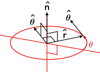
The standard ordered vector basis for spherical polar coordinates;
 are used with the general forms of unit vectors below.
Common general themes of unit vectors occur throughout physics:
Unit vector Nomenclature Diagram Tangent vector to a curve/flux line 
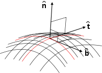
A normal vector
 to the plane containing and defined by the radial position vector
  and angular tangential direction of rotation
  is necessary so that the vector equations of angular motion hold.
Normal to a surface tangent plane/plane containing radial position component and angular tangential component
In terms of polar coordinates;

Binormal vector to tangent and normal  [2]
[2]Parallel to some axis/line 
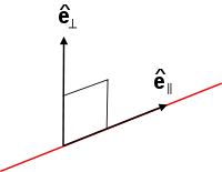
One unit vector
aligned parallel to a principle direction (red line), and a perpendicular unit vector  is in any radial direction relative to the principle line.
Perpendicular to some axis/line in some radial direction Possible angular deviation relative to some axis/line 
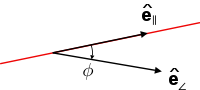
Unit vector at acute deviation angle φ (including 0 or π/2 rad) relative to a principle direction.
Classical mechanics
Mass and inertia
Quantity (common name/s) (Common) symbol/s Defining equation SI units Dimension Linear, surface, volumetric mass density λ or μ (especially in acoustics, see below) for Linear, σ for surface, ρ for volume.  (or
(or  )
)


kg m−n, n = 1, 2, 3 [M][L]−n Moment of mass[3] m (No common symbol) Point mass:

Descrete masses about an axis
 :
:

Continuum of mass about an axis
:

kg m [M][L] Centre of mass rcom (Symbols vary)
ith moment of mass 
Discrete masses:

Mass continuum:

m [L] 2-Body reduced mass m12, μ Pair of masses = m1 and m2 
kg [M][L]2 Moment of inertia (MOI) I Discrete Masses:

Mass continuum:

kg m2 s−1 [M][L]2 Derived kinematic quantities
Quantity (common name/s) (Common) symbol/s Defining equation SI units Dimension Velocity v 
m s−1 [L][T]−1 Acceleration a 
m s−2 [L][T]−2 Jerk j 
m s−3 [L][T]−3 Angular velocity ω 
rad s−1 [T]−1 Angular Acceleration α 
rad s−2 [L][T]−2 Derived dynamic quantities
Quantity (common name/s) (Common) symbol/s Defining equation SI units Dimension Momentum p 
kg m s−1 [M][L][T]−1 Force F 
N = kg m s−2 [M][L][T]−2 Impulse Δp, I 
kg m s−1 [M][L][T]−1 Angular momentum about a position point r0, L, J, S 
Most of the time we can set r0 = 0 if particles are orbiting about axes intersecting at a common point.
kg m2 s−1 [M][L]2[T]−1 Moment of a force about a position point r0, τ, M 
N m = kg m2 s−2 [M][L]2[T]−2 Angular impulse ΔL (no common symbol) 
kg m2 s−1 [M][L]2[T]−1 General energy definitions
Main article: Mechanical energyQuantity (common name/s) (Common) symbol/s Defining equation SI units Dimension Mechanical work due to a Resultant Force
W 
J = N m = kg m2 s−2 [M][L]2[T]−2 Work done ON mechanical system, Work done BY
WON, WBY 
J = N m = kg m2 s−2 [M][L]2[T]−2 Potential energy φ, Φ, U, V, Ep 
J = N m = kg m2 s−2 [M][L]2[T]−2 Mechanical power P 
W = J s−1 [M][L]2[T]−3 Lagrangian L 
J [M][L]2[T]−2 Hamiltonian H 
J [M][L]2[T]−2 Action S, 

J s [M][L]2[T]−1 Every conservative force has a potential energy. By following two principles one can consistently assign a non-relative value to U:
- Wherever the force is zero, its potential energy is defined to be zero as well. - Whenever the force does work, potential energy is lost.
Transport mechanics
Here
is a unit vector in the direction of the flow/current/flux.Quantity (common name/s) (Common) symbol/s Defining equation SI units Dimension Flow velocity vector field u 
m s−1 [L][T]−1 Volume velocity, volume flux φV (no standard symbol) 
m3 s−1 [L]3 [T]−1 Mass current per unit volume s (no standard symbol) 
kg m−3 s−1 [M] [L]−3 [T]−1 Mass current, mass flow rate Im 
kg s−1 [M][T]−1 Mass current density jm 
kg m−2 s−1 [M][L]−2[T]−1 Momentum current Ip 
kg m s−2 [M][L][T]−2 Momentum current density jp 
kg m s−2 [M][L][T]−2 Properties of matter
Stress and strain
Quantity (common name/s) (Common) symbol/s Defining equation SI units Dimension General stress, P, σ 
F may be any force applied to area A
Pa = N m−2 [M] [T] [L]−1 General strain ε 
D = dimension (length, area, volume)
 = change in dimension
dimensionless dimensionless General elastic modulus Emod 
Pa = N m−2 [M] [T] [L]−1 Young's modulus E, Y 
Pa = N m−2 [M] [T] [L]−1 Shear modulus G 
Pa = N m−2 [M] [T] [L]−1 Bulk modulus B 
Pa = N m−2 [M] [T] [L]−1 Compressibility C 
Pa−1 = m2 N−1 [L] [M]−1 [T]−1 Thermodynamics
Thermodynamic quantities
Main articles: List of thermodynamic properties, Thermodynamic potential, Free entropy, Defining equation (physical chemistry)General fundamental quantities
Quantity (common name/s) (Common) symbol/s SI units Dimension Number of molecules N dimensionless dimensionless Number of moles n mol [N] Temperature T K [Θ] Heat energy Q, q J [M][L]2[T]−2 Latent heat QL J [M][L]2[T]−2 Entropy S J K−1 [M][L]2[T]−2 [Θ]−1 Negentropy J J K−1 [M][L]2[T]−2 [Θ]−1 Thermal properties of matter
Main Articles: Heat capacity, Thermal expansionQuantity (common name/s) (Common) symbol/s Defining equation SI units Dimension General heat/thermal capacity C 
J K −1 [M][L]2[T]−2 [Θ]−1 Heat capacity (isobaric) Cp 
J K −1 [M][L]2[T]−2 [Θ]−1 Specific heat capacity (isobaric) Cmp 
J kg−1 K−1 [L]2[T]−2 [Θ]−1 Molar specific heat Capacity (isobaric)
Cnp 
J K −1 mol−1 [M][L]2[T]−2 [Θ]−1 [N]−1 Heat capacity (isochoric/volumetric) CV 
J K −1 [M][L]2[T]−2 [Θ]−1 Specific heat capacity (isochoric) CmV 
J kg−1 K−1 [L]2[T]−2 [Θ]−1 Molar specific heat capacity (isochoric) CnV 
J K −1 mol−1 [M][L]2[T]−2 [Θ]−1 [N]−1 Specific latent heat L 
J kg−1 [L]2[T]−2 Ratio of isobaric to isochoric heat capacity, Heat capacity ratio, adiabatic index
γ 
dimensionless dimensionless Thermal transfer
Main article: Thermal conductivityQuantity (common name/s) (Common) symbol/s Defining equation SI units Dimension Temperature gradient No standard symbol 
K m−1 [Θ][L]−1 Thermal conduction rate, thermal current, thermal/heat flux, thermal power transfer P 
W = J s−1 [M] [L]2 [T]−2 Thermal intensity I 
W m−2 [M] [T]−3 Thermal/heat flux density (vector analogue of thermal intensity above) q 
W m−2 [M] [T]−3 Waves
General fundamental quantities
A wave can be longnitudinal where the oscillations are parallel (or antiparallel) to the propagation direction, or transverse where the oscillations are perpendicular to the propagation direction. These oscillations are characterized by a periodically time-varying displacement in the parallel or perpendicular direction, and so the instantaneous velocity and acceleration are also periodic and time varying in these directions. But the wave profile (the apparent motion of the wave due to the successive oscillations of particles or fields about their equilibrium positions) propagates at the phase and group velocities parallel or antiparallel to the propagation direction, which is common to longitudinal and transverse waves. Below oscillatory displacement, velocity and acceleration refer to the kinematics in the oscillating directions of the wave - transverse or longitudinal (mathematical description is identical), the group and phase velocities are separate.
Main articles: Transverse wave, Longitudinal waveQuantity (common name/s) (Common) symbol/s SI units Dimension Number of wave cycles N dimensionless dimensionless (Oscillatory) displacement Symbol of any quantity which varies periodically, such as h, x, y (mechanical waves), x, s, η (longitudinal waves) I, V, E, B, H, D (electromagnetism), u, U (luminal waves), ψ, Ψ, Φ (quantum mechanics). Most general purposes use y, ψ, Ψ. For generality here, A is used and can be replaced by any other symbol, since others have specific, common uses.  for longitudinal waves,
 for transverse waves.
m [L] (Oscillatory) displacement amplitude Any quantity symbol typically subscripted with 0, m or max, or the capitalized letter (if displacement was in lower case). Here for generality A0 is used and can be replaced. m [L] (Oscillatory) velocity amplitude V, v0, vm. Here v0 is used. m s−1 [L][T]−1 (Oscillatory) acceleration amplitude A, a0, am. Here a0 is used. m s−2 [L][T]−2 Spatial position
Position of a point in space, not necessarily a point on the wave profile or any line of propagationd, r m [M] Wave profile displacement
Along propagation direction, distance travelled (path length) by one wave from the source point r0 to any point in space d (for longitudinal or transverse waves)L, d, r 
m [L] Phase angle δ, ε, φ rad dimensionless General derived quantities
Quantity (common name/s) (Common) symbol/s Defining equation SI units Dimension Wavelength λ General definition (allows for FM):

For non-FM waves this reduces to:

m [L] Wavenumber, k-vector, Wave vector k, σ Two definitions are in use:


m−1 [L]−1 Frequency f, ν General definition (allows for FM):

For non-FM waves this reduces to:

In practice N is set to 1 cycle and t = T = time period for 1 cycle, to obtain the more useful relation:

Hz = s−1 [T]−1 Angular frequency/ pulsatance ω 
Hz = s−1 [T]−1 Oscillatory velocity v, vt, v Longitudinal waves:

Transverse waves:

m s−1 [L][T]−1 Oscillatory acceleration a, at Longitudinal waves:

Transverse waves:

m s−2 [L][T]−2 Path length difference between two waves L, ΔL, Δx, Δr 
m [L] Phase velocity vp General definition:

In practice reduces to the useful form:

m s−1 [L][T]−1 (Longitudinal) group velocity vg 
m s−1 [L][T]−1 Time delay, time lag/lead Δt 
s [T] Phase difference δ, Δε, Δϕ 
rad dimensionless Phase No standard symbol 
Physically;
upper sign: wave propagation in +r direction
lower sign: wave propagation in −r directionPhase angle can lag if: ϕ > 0
or lead if: ϕ < 0.rad dimensionless Relation between space, time, angle analogues used to describe the phase:

Modulation indicies
Quantity (common name/s) (Common) symbol/s Defining equation SI units Dimension AM index: h, hAM 
A = carrier amplitude
Am = peak amplitude of a component in the modulating signaldimensionless dimensionless FM index: hFM 
Δf = max. deviation of the instantaneous frequency from the carrier frequency
fm = peak frequency of a component in the modulating signaldimensionless dimensionless PM index: hPM 
Δϕ = peak phase deviation
dimensionless dimensionless Acoustics
Quantity (common name/s) (Common) symbol/s Defining equation SI units Dimension Acoustic impedance Z 
v = speed of sound, ρ = volume density of medium
kg m−2 s−1 [M] [L]−2 [T]−1 Specific acoustic impedance z 
S = surface area
kg s−1 [M] [T]−1 Sound Level β 
dimensionless dimensionless Gravitation
A common misconseption occurs between centre of mass and centre of gravity. They are defined in similar ways but are not exactly the same quantity. Centre of mass is the mathematical descrition of placing all the mass in the region considered to one position, centre of gravity is a real physical quantity, the point of a body where the gravitational force acts. They are only equal if and only if the external gravitational field is uniform.
Quantity (common name/s) (Common) symbol/s Defining equation SI units Dimension Centre of gravity rcog (symbols vary) ith moment of mass 
Centre of gravity for a descrete masses:

Centre of a gravity for a continuum of mass:

m [L] Standard gravitational parameter of a mass μ 
N m2 kg−1 [L]3 [T]−2 Gravitational field, field strength, potential gradient, acceleration g 
N kg−1 = m s−2 [L][T]−2 Gravitational flux ΦG 
m3 s−2 [L]3[T]−2 Absolute gravitational potential Φ, φ, U, V 
J kg−1 [L]2[T]−2 Gravitational potential difference ΔΦ, Δφ, ΔU, ΔV 
J kg−1 [L]2[T]−2 Gravitational potential energy Ep 
J [M][L]2[T]−2 Gravitational torsion field Ω 
Hz = s−1 [T]−1 Gravitational torsion flux ΦΩ 
N m s kg−1 = m2 s−1 [M]2 [T]−1 Gravitomagnetic field H, Bg, B, ξ 
Hz = s−1 [T]−1 Gravitomagnetic flux Φξ 
N m s kg−1 = m2 s−1 [M]2 [T]−1 Gravitomagnetic vector potential [4] h 
m s−1 [M] [T]−1 Electromagnetism
Here subscripts e and m are used to differ between electric and magnetic charges. The definitions for monopoles are of theoretical interest, although real magnetic dipoles can be described using pole strengths. There are two possible units for monopole strength, Wb (Weber) and A m (Ampere metre). Dimensional analysis shows that magnetic charges relate by qm(Wb) = μ0 qm(Am).
Initial quantities
Quantity (common name/s) (Common) symbol/s SI units Dimension Electric charge qe, q, Q C = As [I][T] Monopole strength, magnetic charge qm, g, p Wb or Am [L]2[M][T]−2 [I]−1 (Wb)
[I][L] (Am)
Electric quantities
Contrary to the strong analogy between (classical) gravitation and electrostatics, there are no "centre of charge" or "centre of electrostatic attraction" analogues.
Electric transport
Quantity (common name/s) (Common) symbol/s Defining equation SI units Dimension Linear, surface, volumetric charge density λe for Linear, σe for surface, ρe for volume. 


C m−n, n = 1, 2, 3 [I][T][L]−n Capacitance C 
V = voltage, not volume.
F = C V−1 [I][T]3[L]−2[M]−1 Electric current I 
A [I] Electric current density J 
A m−2 [I][L]−2 Displacement current density Jd 
Am−2 [I][L]m−2 Convection current density Jc 
A m−2 [I] [L]m−2 Electric fields
Quantity (common name/s) (Common) symbol/s Defining equation SI units Dimension Electric field, field strength, flux density, potential gradient E 
N C−1 = V m−1 [M][L][T]−3[I]−1 Electric flux ΦE 
N m2 C−1 [M][L]3[T]−3[I]−1 Absolute permittivity; ε 
F m−1 [I]2 [T]4 [M]−1 [L]−3 Electric displacement field D 
C m−2 [I][T][L]−2 Electric displacement flux ΦD 
C [I][T] Electric dipole moment p 
a = charge separation directed from -ve to +ve charge
C m [I][T][L] Electric Polarization, polarization density P 
C m−2 [I][T][L]−2 Absolute electric potential, EM scalar potential relative to point 
Theoretical:

Practical: (Earth's radius)
φ ,V 
V = J C−1 [M] [L] [T]−3 [I]−1 Voltage, Electric potential difference Δφ,ΔV 
V = J C−1 [M] [L] [T]−3 [I]−1 Electric potential energy U 
J [M][L]2[T]2 Magnetic quantities
Magnetic transport
Quantity (common name/s) (Common) symbol/s Defining equation SI units Dimension Linear, surface, volumetric pole density λm for Linear, σm for surface, ρm for volume. 


Wb m−n
A m−(n + 1),
n = 1, 2, 3[L]2[M][T]−2 [I]−1 (Wb)
[I][L] (Am)
Monopole current Im 
Wb s−1
A m s−1
[L]2[M][T]−3 [I]−1 (Wb)
[I][L][T]−1 (Am)
Monopole current density Jm 
Wb s−1 m−2
A m−1 s−1
[M][T]−3 [I]−1 (Wb)
[I][L]−1[T]−1 (Am)
Magnetic fields
Quantity (common name/s) (Common) symbol/s Defining equation SI units Dimension Magnetic field, field strength, flux density, induction field B 
T = N A−1 m−1 = Wb m2 [M][T]−2[I]−1 Magnetic potential, EM vector potential A 
T m = N A−1 = Wb m3 [M][L][T]−2[I]−1 Magnetic flux ΦB 
Wb = T m−2 [L]2[M][T]−2[I]−1 Magnetic field intensity, (AKA field strength) H 
A m−1 [I] [L]−1 Magnetic moment, magnetic dipole moment m, μ, Π Two definitions are possible:
using pole strengths,

using currents:

a = pole separation N is the number of turns of conductor
A m2 [I][L]2 Magnetization M 
A m2 [I] [L]−1 Intensity of magnetization, magnetic polarization I, J 
T = N A−1 m−1 = Wb m2 [M][T]−2[I]−1 Self Inductance L Two equivalent definitions are possible: 

H = Wb A−1 [L]2 [M] [T]−2 [I]−2 Mutual inductance M Again two equivalent definitions are possible: 

1,2 subscripts refer to two conductors/inductors mutually inducing voltage/ linking magnetic flux though each other. They can be interchanged for the required conductor/inductor;


H = Wb A−1 [L]2 [M] [T]−2 [I]−2 Gyromagnetic ratio (for charged particles in a magnetic field) γ 
Hz T−1 [M]−1[T][I] Electric circuits
DC circuits, general definitions
Main article: Direct currentQuantity (common name/s) (Common) symbol/s Defining equation SI units Dimension Terminal Voltage for Vter V = J C−1 [M] [L]2 [T]−3 [I]−1 Load Voltage for Circuit Vload V = J C−1 [M] [L]2 [T]−3 [I]−1 Internal resistance of power supply Rint 
Ω = V A−1 = J s C−2 [M][L]2 [T]−3 [I]−2 Load resistance of circuit Rext 
Ω = V A−1 = J s C−2 [M][L]2 [T]−3 [I]−2 Electromotive force (emf), voltage across entire circuit including power supply, external components and conductors E 
V = J C−1 [M] [L]2 [T]−3 [I]−1 AC circuits
Main articles: Alternating current, ResonanceQuantity (common name/s) (Common) symbol/s Defining equation SI units Dimension Resistive load voltage VR 
V = J C−1 [M] [L]2 [T]−3 [I]−1 Capacitive load coltage VC 
V = J C−1 [M] [L]2 [T]−3 [I]−1 Inductive load coltage VL 
V = J C−1 [M] [L]2 [T]−3 [I]−1 Capacitive reactance XC 
Ω−1 m−1 [I]2 [T]3 [M]−2 [L]−2 Inductive reactance XL 
Ω−1 m−1 [I]2 [T]3 [M]−2 [L]−2 AC electrical impedance Z 

Ω−1 m−1 [I]2 [T]3 [M]−2 [L]−2 Phase constant δ, φ 
dimensionless dimensionless AC peak current I0 
A [I] AC root mean square current Irms ![I_\mathrm{rms} = \sqrt{\frac{1}{T} \int_{0}^{T} \left [ I \left ( t \right ) \right ]^2 \mathrm{d} t} \,\!](c/3dc612366a1a6a3ae60a4d72d53c0767.png)
A [I] AC peak voltage V0 
V = J C−1 [M] [L]2 [T]−3 [I]−1 AC root mean square voltage Vrms ![V_\mathrm{rms} = \sqrt{\frac{1}{T} \int_{0}^{T} \left [ V \left ( t \right ) \right ]^2 \mathrm{d} t} \,\!](d/d0db1de2c13f2b62e6544e8171212c03.png)
V = J C−1 [M] [L]2 [T]−3 [I]−1 AC emf, root mean square 

V = J C−1 [M] [L]2 [T]−3 [I]−1 AC average power 

W = J s−1 [M] [L]2 [T]−3 Capacitive time constant τC 
s [T] Inductive time constant τL 
s [T] Magnetic circuits
Main article: Magnetic circuitsQuantity (common name/s) (Common) symbol/s Defining equation SI units Dimension Magnetomotive force, mmf F, 

N = number of turns of conductor
A [I] Photonics
Geometric optics (luminal rays)
Main article: Geometrical opticsGeneral fundamental quantities
Quantity (common name/s) (Common) symbol/s SI units Dimension Object distance x, s, d, u, x1, s1, d1, u1 m [L] Image distance x', s', d', v, x2, s2, d2, v2 m [L] Object height y, h, y1, h1 m [L] Image height y', h', H, y2, h2, H2 m [L] Angle subtended by object θ, θo, θ1 rad dimensionless Angle subtended by image θ', θi, θ2 rad dimensionless Curvature radius of lens/mirror r, R m [L] Focal length f m [L] Quantity (common name/s) (Common) symbol/s Defining equation SI units Dimension Lens power P 
m−1 = D (dioptre) [L]−1 Lateral magnification m 
dimensionless dimensionless Angular magnification m 
dimensionless dimensionless Physical optics (EM luminal waves)
Main article: Physical opticsThere are different forms of the Poynting vector, the most common are in terms of the E and B or E and H fields.
Quantity (common name/s) (Common) symbol/s Defining equation SI units Dimension Poynting vector S, N 
W m−2 [M][T]−3 Poynting flux, EM field power flow ΦS, ΦN 
W [M][L]2[T]−3 RMS Electric field of Light Erms 
N C−1 = V m−1 [M][L][T]−3[I]−1 Radiation momentum p, pEM, pr 
J s m−1 [M][L][T]−1 Radiation pressure Pr, pr, PEM 
W m−2 [M][T]−3 Radiometry
Main article: Radiometry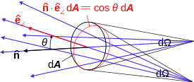 Visulization of flux through differential area and solid angle. As always
 is the unit normal to the incidant surface A,
  , and is a unit vector in the direction of incident flux on the area element, θ is the angle between them. The factor
  arises when the flux is not normal to the surface element, so the area normal to the flux is reduced.
For spectral quantities two definitions are in use to refer to the same quantity, in terms of frequency or wavelength.
Quantity (common name/s) (Common) symbol/s Defining equation SI units Dimension Radiant energy Q, E, Qe, Ee J [M][L]2[T]−2 Radiant exposure He 
J m−2 [M][T]−3 Radiant energy density ωe 
J m−3 [M][L]−3 Radiant flux, radiant power Φ, Φe 
W [M][L]2[T]−3 Radiant intensity I, Ie 
W sr−1 [M][L]2[T]−3 Radiance, intensity L, Le 
W sr−1 m−2 [M][T]−3 Irradiance E, I, Ee, Ie 
W m−2 [M][T]−3 Radiant exitance, radiant emittance M, Me 
W m−2 [M][T]−3 Radiosity J, Jν, Je, Jeν 
W m−2 [M][T]−3 Spectral radiant flux, spectral radiant power Φλ, Φν, Φeλ, Φeν 
W m−1 (Φλ)
W Hz−1 = J (Φν)[M][L]−3[T]−3 (Φλ)
[M][L]−2[T]−2 (Φν)Spectral radiant intensity Iλ, Iν, Ieλ, Ieν 
W sr−1 m−1 (Iλ)
W sr−1 Hz−1 (Iν)[M][L]−3[T]−3 (Iλ)
[M][L]2[T]−2 (Iν)Spectral radiance Lλ, Lν, Leλ, Leν 
W sr−1 m−3 (Lλ)
W sr−1 m−2 Hz−1 (Lν)[M][L]−1[T]−3 (Lλ)
[M][L]−2[T]−2 (Lν)Spectral irradiance Eλ, Eν, Eeλ, Eeν 
W m−3 (Eλ)
W m−2 Hz−1 (Eν)[M][L]−1[T]−3 (Eλ)
[M][L]−2[T]−2 (Eν)Atomic/nuclear physics
Quantity (common name/s) (Common) symbol/s Defining equation SI units Dimension Number of atoms N = Number of atoms remaining at time t
N0 = Initial number of atoms at time t = 0
ND = Number of atoms decayed at time t
dimensionless dimensionless Decay rate, activity of a radioisotope A 
Bq = Hz = s−1 [T]−1 Decay constant λ 
Bq = Hz = s−1 [T]−1 Half-life of a radioisotope t1/2, T1/2 Time taken for half the number of atoms present to decay 

s [T] Number of half-lives n (no standard symbol) 
dimensionless dimensionless Radioisotope time constant, mean lifetime of an atom before decay τ (no standard symbol) 
s [T] Absorbed dose, total ionizing dose (total energy of radiation transferred to unit mass) D can only be found experimentally N/A Sv = J kg−1 (Sievert) [L]2[T]−2 Equivalent dose H 
Q = radiation quality factor (dimensionless)
Sv = J kg−1 (Sievert) [L]2[T]−2 Effective dose E 
Wj = weighting factors corresponding to radiosensitivities of matter (dimensionless)

Sv = J kg−1 (Sievert) [L]2[T]−2 Quantum mechanics
Quantity (common name/s) (Common) symbol/s Defining equation SI units Dimension Wave function ψ, Ψ To solve from the Schrödinger equation varies with situation and number of particles Threshold frequency f0, ν0 Can only be found by experiment/calculated from work function below. Hz = s−1 [T]−1 Work function φ, Φ 
J [M][L]2[T]−2 Wavefunction probability density ρ 
m−3 [L]−3 Wavefunction probability current j Non-relativistic, no external field: 

star * is complex conjugate
m−2 s−1 [T]−1 [L]−2 Astrophysics
In astrophysics, L is used for luminosity (energy per unit time, equivalent to power) and F is used for energy flux (energy per unit time per unit area, equivalent to intensity in terms of area, not solid angle). They are not new quantities, simply different names.
Quantity (common name/s) (Common) symbol/s Defining equation SI units Dimension Comoving transverse distance DM pc (parsecs) [L] Luminosity distance DL 
pc (parsecs) [L] Apparent magnitude in band j (UV, visible and IR parts of EM spectrum) (Bolometric) m 
dimensionless dimensionless Absolute magnitude (Bolometric)
M ![M = m - 5 \left [ \left ( \log_{10}{D_L} \right ) - 1 \right ]\!\,](6/2a6ffe3a78bc638b62716a989bda4fd3.png)
dimensionless dimensionless Distance modulus μ 
dimensionless dimensionless Colour indices (No standard symbols) 

dimensionless dimensionless Bolometric correction Cbol (No standard symbol) 
dimensionless dimensionless See also
List of physics formulae
Defining equation (physical chemistry)Footnotes
- ^ Warlimont, pp 12–13
- ^ Vector Analysis (2nd Edition), Schaum's Outlines Series, M. R. Spiegel, S. Lipschutz, D. Spellman, Mc Graw Hill, ISBN 978 0 07 161545 7
- ^ http://www.ltcconline.net/greenl/courses/202/multipleIntegration/MassMoments.htm, Section: Moments and center of mass
- ^ Gravitation and Inertia, I. Ciufolini and J.A. Wheeler, Princeton Physics Series, 1995, ISBN 0-691-03323-4
References
- Dynamics and Relativity, J.R. Forshaw, A.G. Smith, Wiley, 2009, ISBN 978 0 470 01460 8
- Essential Principles of Physics, P.M. Whelan, M.J. Hodgeson, 2nd Edition, 1978, John Murray, ISBN 0 7195 3382 1
- Encyclopaedia of Physics, R.G. Lerner, G.L. Trigg, 2nd Edition, VHC Publishers, Hans Warlimont, Springer, 2005, pp 12–13
- Physics for Scientists and Engineers: With Modern Physics (6th Edition), P.A. Tipler, G. Mosca, W.H. Freeman and Co, 2008, 9-781429-202657
SI units Base units 
Derived units Accepted for use
with SIDalton (Atomic mass unit) · Astronomical unit · Day · Decibel · Degree of arc · Electronvolt · Hectare · Hour · Litre · Minute · Minute of arc · Neper · Second of arc · Tonne
Atomic units · Natural unitsSee also SI prefixes · Systems of measurement · Conversion of units · New SI definitions · History of the metric system Book:International System of Units ·
  Category:SI base unitsCategories:
- Measurement
- Physics
- Mathematical physics
- Physical quantities
- SI base units
- SI derived units
- SI units
- Physical chemistry


Wikimedia Foundation. 2010.