- Chebyshev polynomials
-
Not to be confused with discrete Chebyshev polynomials.
In mathematics the Chebyshev polynomials, named after Pafnuty Chebyshev,[1] are a sequence of orthogonal polynomials which are related to de Moivre's formula and which can be defined recursively. One usually distinguishes between Chebyshev polynomials of the first kind which are denoted Tn and Chebyshev polynomials of the second kind which are denoted Un. The letter T is used because of the alternative transliterations of the name Chebyshev as Tchebycheff (French) or Tschebyschow (German).
The Chebyshev polynomials Tn or Un are polynomials of degree n and the sequence of Chebyshev polynomials of either kind composes a polynomial sequence.
Chebyshev polynomials are important in approximation theory because the roots of the Chebyshev polynomials of the first kind, which are also called Chebyshev nodes, are used as nodes in polynomial interpolation. The resulting interpolation polynomial minimizes the problem of Runge's phenomenon and provides an approximation that is close to the polynomial of best approximation to a continuous function under the maximum norm. This approximation leads directly to the method of Clenshaw–Curtis quadrature.
In the study of differential equations they arise as the solution to the Chebyshev differential equations
and
for the polynomials of the first and second kind, respectively. These equations are special cases of the Sturm–Liouville differential equation.
Contents
Definition
The Chebyshev polynomials of the first kind are defined by the recurrence relation
The conventional generating function for Tn is
The exponential generating function is
The Chebyshev polynomials of the second kind are defined by the recurrence relation
One example of a generating function for Un is
Trigonometric definition
The Chebyshev polynomials of the first kind can be defined by the trigonometric identity:
whence:
for n = 0, 1, 2, 3, ..., while the polynomials of the second kind satisfy:
which is structurally quite similar to the Dirichlet kernel
 :
:That cos(nx) is an nth-degree polynomial in cos(x) can be seen by observing that cos(nx) is the real part of one side of de Moivre's formula, and the real part of the other side is a polynomial in cos(x) and sin(x), in which all powers of sin(x) are even and thus replaceable via the identity cos2(x) + sin2(x) = 1.
This identity is extremely useful in conjunction with the recursive generating formula inasmuch as it enables one to calculate the cosine of any integral multiple of an angle solely in terms of the cosine of the base angle. Evaluating the first two Chebyshev polynomials:
and:
one can straightforwardly determine that:
and so forth.
Two immediate corollaries are the composition identity (or the "nesting property")
and the expression of complex exponentiation in terms of Chebyshev polynomials: given z = a + bi,
Pell equation definition
The Chebyshev polynomials can also be defined as the solutions to the Pell equation
in a ring R[x].[2] Thus, they can be generated by the standard technique for Pell equations of taking powers of a fundamental solution:
Relation between Chebyshev polynomials of the first and second kinds
The Chebyshev polynomials of the first and second kind are closely related by the following equations
 , where n is odd.
 , where n is even.
The recurrence relationship of the derivative of Chebyshev polynomials can be derived from these relations
This relationship is used in the Chebyshev spectral method of solving differential equations.
Equivalently, the two sequences can also be defined from a pair of mutual recurrence equations:
These can be derived from the trigonometric formulae; for example, if
 , then
Note that both these equations and the trigonometric equations take a simpler form if we, like some works, follow the alternate convention of denoting our Un (the polynomial of degree n) with Un+1 instead.
Turán's inequalities for the Chebyshev polynomials are
 and
and
Explicit formulas
Different approaches to defining Chebyshev polynomials lead to different explicit formulas such as:
where 2F1 is a hypergeometric function.
Properties
Roots and extrema
A Chebyshev polynomial of either kind with degree n has n different simple roots, called Chebyshev roots, in the interval [−1,1]. The roots are sometimes called Chebyshev nodes because they are used as nodes in polynomial interpolation. Using the trigonometric definition and the fact that
one can easily prove that the roots of Tn are
Similarly, the roots of Un are
One unique property of the Chebyshev polynomials of the first kind is that on the interval −1 ≤ x ≤ 1 all of the extrema have values that are either −1 or 1. Thus these polynomials have only two finite critical values, the defining property of Shabat polynomials. Both the first and second kinds of Chebyshev polynomial have extrema at the endpoints, given by:
Differentiation and integration
The derivatives of the polynomials can be less than straightforward. By differentiating the polynomials in their trigonometric forms, it's easy to show that:
The last two formulas can be numerically troublesome due to the division by zero (0/0 indeterminate form, specifically) at x = 1 and x = −1. It can be shown that:
ProofThe second derivative of the Chebyshev polynomial of the first kind is
which, if evaluated as shown above, poses a problem because it is indeterminate at x = ±1. Since the function is a polynomial, (all of) the derivatives must exist for all real numbers, so the taking to limit on the expression above should yield the desired value:
where only x = 1 is considered for now. Factoring the denominator:
Since the limit as a whole must exist, the limit of the numerator and denominator must independently exist, and
The denominator (still) limits to zero, which implies that the numerator must be limiting to zero, i.e. Un − 1(1) = nTn(1) = n which will be useful later on. Since the numerator and denominator are both limiting to zero, L'Hôpital's rule applies:
The proof for x = − 1 is similar, with the fact that Tn( − 1) = ( − 1)n being important.
Indeed, the following, more general formula holds:
This latter result is of great use in the numerical solution of eigenvalue problems.
Concerning integration, the first derivative of the Tn implies that
and the recurrence relation for the first kind polynomials involving derivatives establishes that
Orthogonality
Both the Tn and the Un form a sequence of orthogonal polynomials. The polynomials of the first kind are orthogonal with respect to the weight
on the interval (−1,1), i.e. we have:
This can be proven by letting
 and using the identity
  .
.Similarly, the polynomials of the second kind are orthogonal with respect to the weight
on the interval [−1,1], i.e. we have:
(Note that the weight
 is, to within a normalizing constant, the density of the Wigner semicircle distribution).
The Tn also satisfy a discrete orthogonality condition:
where the xk are the N Gauss–Lobatto zeros of TN(x)
Minimal ∞-norm
For any given n ≥ 1, among the polynomials of degree n with leading coefficient 1,
is the one of which the maximal absolute value on the interval [−1, 1] is minimal.
This maximal absolute value is
and |ƒ(x)| reaches this maximum exactly n + 1 times at
Proof
Let's assume that wn(x) is a polynomial of degree n with leading coefficient 1 with maximal absolute value on the interval [−1, 1] less than
 .
.We define
Because at extreme points of Tn we have

From the intermediate value theorem, fn(x) has at least n roots. However, this is impossible, as fn(x) is a polynomial of degree n − 1, so the fundamental theorem of algebra implies it has at most n − 1 roots.
Other properties
The Chebyshev polynomials are a special case of the ultraspherical or Gegenbauer polynomials, which themselves are a special case of the Jacobi polynomials:
For every nonnegative integer n, Tn(x) and Un(x) are both polynomials of degree n. They are even or odd functions of x as n is even or odd, so when written as polynomials of x, it only has even or odd degree terms respectively. In fact,
and
The leading coefficient of Tn is 2n − 1 if 1 ≤ n, but 1 if 0 = n.
Tn are a special case of Lissajous curves with frequency ratio equal to n.
Several polynomial sequences like Lucas polynomials (Ln), Dickson polynomials(Dn), Fibonacci polynomials(Fn) are related to Chebyshev polynomials Tn and Un.
The Chebyshev polynomials of the first kind satisfy the relation
which is easily proved from the product-to-sum formula for the cosine. The polynomials of the second kind satisfy the similar relation
 .
.
Similar to the formula
- Tn(cos θ) = cos(nθ)
we have the analogous formula
- T2n + 1(sin θ) = ( − 1)nsin((2n + 1)θ).
Let
 .
.
Then Cn(x) and Cm(x) are commuting polynomials:
- Cn(Cm(x)) = Cm(Cn(x)).
Examples
 The first few Chebyshev polynomials of the first kind in the domain −1 < x < 1: The flat T0, T1, T2, T3, T4 and T5.
The first few Chebyshev polynomials of the first kind are
 The first few Chebyshev polynomials of the second kind in the domain −1 < x < 1: The flat U0, U1, U2, U3, U4 and U5. Although not visible in the image, Un(1) = n + 1 and Un(−1) = (n + 1)(−1)n.
The first few Chebyshev polynomials of the second kind are
As a basis set
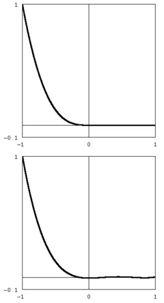 The non-smooth function (top) y = −x3H(−x), where H is the Heaviside step function, and (bottom) the 5th partial sum of its Chebyshev expansion. The 7th sum is indistinguishable from the original function at the resolution of the graph.
In the appropriate Sobolev space, the set of Chebyshev polynomials form a complete basis set, so that a function in the same space can, on −1 ≤ x ≤ 1 be expressed via the expansion:[3]
Furthermore, as mentioned previously, the Chebyshev polynomials form an orthogonal basis which (among other things) implies that the coefficients an can be determined easily through the application of an inner product. This sum is called a Chebyshev series or a Chebyshev expansion.
Since a Chebyshev series is related to a Fourier cosine series through a change of variables, all of the theorems, identities, etc. that apply to Fourier series have a Chebyshev counterpart.[3] These attributes include:
- The Chebyshev polynomials form a complete orthogonal system.
- The Chebyshev series converges to ƒ(x) if the function is piecewise smooth and continuous. The smoothness requirement can be relaxed in most cases — as long as there are a finite number of discontinuities in ƒ(x) and its derivatives.
- At a discontinuity, the series will converge to the average of the right and left limits.
The abundance of the theorems and identities inherited from Fourier series make the Chebyshev polynomials important tools in numeric analysis; for example they are the most popular general purpose basis functions used in the spectral method,[3] often in favor of trigonometric series due to generally faster convergence for continuous functions (Gibbs' phenomenon is still a problem).
Example 1
Consider the Chebyshev expansion of log(1 + x). One can express
One can find the coefficients an either through the application of an inner product or by the discrete orthogonality condition. For the inner product,
which gives
Alternatively, when you cannot evaluate the inner product of the function you are trying to approximate, the discrete orthogonality condition gives
where δij is the Kronecker delta function and the xk are the N Gauss–Lobatto zeros of TN(x)
This allows us to compute the coefficients an very efficiently through the discrete cosine transform
Example 2
To provide another example:
Partial sums
The partial sums of
are very useful in the approximation of various functions and in the solution of differential equations (see spectral method). Two common methods for determining the coefficients an are through the use of the inner product as in Galerkin's method and through the use of collocation which is related to interpolation.
As an interpolant, the N coefficients of the (N − 1)th partial sum are usually obtained on the Chebyshev–Gauss–Lobatto[4] points (or Lobatto grid), which results in minimum error and avoids Runge's phenomenon associated with a uniform grid. This collection of points corresponds to the extrema of the highest order polynomial in the sum, plus the endpoints and is given by:
Polynomial in Chebyshev form
An arbitrary polynomial of degree N can be written in terms of the Chebyshev polynomials of the first kind. Such a polynomial p(x) is of the form
Polynomials in Chebyshev form can be evaluated using the Clenshaw algorithm.
Spread polynomials
The spread polynomials are in a sense equivalent to the Chebyshev polynomials of the first kind, but enable one to avoid square roots and conventional trigonometric functions in certain contexts, notably in rational trigonometry.
See also
- Chebyshev nodes
- Chebyshev filter
- Chebyshev cube root
- Dickson polynomials
- Legendre polynomials
- Hermite polynomials
- Chebyshev rational functions
- Clenshaw–Curtis quadrature
- Approximation theory
- The Chebfun system
Notes
- ^ Chebyshev polynomials were first presented in: P. L. Chebyshev (1854) "Théorie des mécanismes connus sous le nom de parallélogrammes," Mémoires des Savants étrangers présentés à l’Académie de Saint-Pétersbourg, vol. 7, pages 539–586.
- ^ Jeroen Demeyer Diophantine Sets over Polynomial Rings and Hilbert's Tenth Problem for Function Fields, Ph.D. theses (2007), p.70.
- ^ a b c Boyd, John P. (2001). Chebyshev and Fourier Spectral Methods (second ed.). Dover. ISBN 0486411834. http://www-personal.umich.edu/~jpboyd/aaabook_9500may00.pdf.
- ^ Chebyshev Interpolation: An Interactive Tour
References
- Abramowitz, Milton; Stegun, Irene A., eds. (1965), "Chapter 22", Handbook of Mathematical Functions with Formulas, Graphs, and Mathematical Tables, New York: Dover, pp. 773, ISBN 978-0486612720, MR0167642, http://www.math.sfu.ca/~cbm/aands/page_773.htm.
- Koornwinder, Tom H.; Wong, Roderick S. C.; Koekoek, Roelof; Swarttouw, René F. (2010), "Orthogonal Polynomials", in Olver, Frank W. J.; Lozier, Daniel M.; Boisvert, Ronald F. et al., NIST Handbook of Mathematical Functions, Cambridge University Press, ISBN 978-0521192255, MR2723248, http://dlmf.nist.gov/18
- Suetin, P.K. (2001), "Chebyshev polynomials", in Hazewinkel, Michiel, Encyclopaedia of Mathematics, Springer, ISBN 978-1556080104, http://eom.springer.de/C/c021940.htm
External links
- Weisstein, Eric W., "Chebyshev Polynomial of the First Kind" from MathWorld.
- Module for Chebyshev Polynomials by John H. Mathews
- Chebyshev Interpolation: An Interactive Tour, includes illustrative Java applet.
- Numerical Computing with Functions: The Chebfun Project
Categories:- Polynomials
- Special hypergeometric functions
- Orthogonal polynomials
- Numerical analysis
- Approximation theory


![T_n(x) =
\begin{cases}
\cos(n\arccos(x)), & \ x \in [-1,1] \\
\cosh(n \, \mathrm{arccosh}(x)), & \ x \ge 1 \\
(-1)^n \cosh(n \, \mathrm{arccosh}(-x)), & \ x \le -1 \\
\end{cases} \,\!](8/298db80c31f00d2887358dc3107aadd7.png)


Wikimedia Foundation. 2010.