- RLC circuit
-
 A series RLC circuit: a resistor, inductor, and a capacitor
An RLC circuit (or LCR circuit) is an electrical circuit consisting of a resistor, an inductor, and a capacitor, connected in series or in parallel. The RLC part of the name is due to those letters being the usual electrical symbols for resistance, inductance and capacitance respectively. The circuit forms a harmonic oscillator for current and will resonate in just the same way as an LC circuit will. The difference that the presence of the resistor makes is that any oscillation induced in the circuit will die away over time if it is not kept going by a source. This effect of the resistor is called damping. Some resistance is unavoidable in real circuits, even if a resistor is not specifically included as a component. A pure LC circuit is an ideal which really only exists in theory.
There are many applications for this circuit. They are used in many different types of oscillator circuit. Another important application is for tuning, such as in radio receivers or television sets, where they are used to select a narrow range of frequencies from the ambient radio waves. In this role the circuit is often referred to as a tuned circuit. An RLC circuit can be used as a band-pass filter or a band-stop filter. The tuning application, for instance, is an example of band-pass filtering. The RLC filter is described as a second-order circuit, meaning that any voltage or current in the circuit can be described by a second-order differential equation in circuit analysis.
The three circuit elements can be combined in a number of different topologies. All three elements in series or all three elements in parallel are the simplest in concept and the most straightforward to analyse. There are, however, other arrangements, some with practical importance in real circuits. One issue often encountered is the need to take into account inductor resistance. Inductors are typically constructed from coils of wire, the resistance of which is not usually desirable, but it often has a significant effect on the circuit.
Contents
Basic concepts
Linear analog electronic filters edit Resonance
An important property of this circuit is its ability to resonate at a specific frequency, the resonance frequency,
 . Frequencies are measured in units of hertz. In this article, however, angular frequency,
  , is used which is more mathematically convenient. This is measured in radians per second. They are related to each other by a simple proportion,
Resonance occurs because energy is stored in two different ways: in an electric field as the capacitor is charged and in a magnetic field as current flows through the inductor. Energy can be transferred from one to the other within the circuit and this can be oscillatory. A mechanical analogy is a weight suspended on a spring which will oscillate up and down when released. This is no passing metaphor, a weight on a spring is described by exactly the same second order differential equation as an RLC circuit and for all the properties of the one system there will be found an analogous property of the other. The mechanical property answering to the resistor in the circuit is friction in the spring/weight system. Friction will slowly bring any oscillation to a halt if there is no external force driving it. Likewise, the resistance in an RLC circuit will "damp" the oscillation, diminishing it with time if there is no driving AC power source in the circuit.
The resonance frequency is defined as the frequency at which the impedance of the circuit is at a minimum. Equivalently, it can be defined as the frequency at which the impedance is purely real (that is, purely resistive). This occurs because the impedance of the inductor and capacitor at resonance are equal but of opposite sign and cancel out. Circuits where L and C are in parallel rather than series actually have a maximum impedance rather than a minimum impedance. For this reason they are often described as antiresonators, it is still usual, however, to name the frequency at which this occurs as the resonance frequency.
Natural frequency
The resonance frequency is defined in terms of the impedance presented to a driving source. It is still possible for the circuit to carry on oscillating (for a time) after the driving source has been removed or it is subjected to a step in voltage (including a step down to zero). This is similar to the way that a tuning fork will carry on ringing after it has been struck, and the effect is often called ringing. This effect is the undriven natural resonance frequency of the circuit and in general is not exactly the same as the driven resonance frequency, although the two will usually be quite close to each other. Various terms are used by different authors to distinguish the two, but resonance frequency unqualified usually means the driven resonance frequency. The driven frequency may be called the undamped resonance frequency or undamped natural frequency and the undriven frequency may be called the damped resonance frequency or the damped natural frequency. The reason for this terminology is that the driven resonance frequency in a series or parallel resonant circuit has the value[1]
This is exactly the same as the resonance frequency of an LC circuit, that is, one with no resistor present, that is, it is the same as a circuit in which there is no damping, hence undamped resonance frequency. The undriven resonance frequency, on the other hand, depends on the value of the resistor and hence is described as the damped resonance frequency. A highly damped circuit will fail to resonate at all when undriven. A circuit with a value of resistor that causes it to be just on the edge of ringing is called critically damped. Either side of critically damped are described as underdamped (ringing happens) and overdamped (ringing is suppressed).
Circuits with topologies more complex than straightforward series or parallel (some examples described later in the article) have a driven resonance frequency that deviates from
 and for those the undamped resonance frequency, damped resonance frequency and driven resonance frequency can all be different.
Damping
Damping is caused by the resistance in the circuit. It determines whether or not the circuit will resonate naturally (that is, without a driving source). Circuits which will resonate in this way are described as underdamped and those that will not are overdamped. Damping attenuation (symbol α) is measured in nepers per second. However, the unitless damping factor (symbol ζ) is often a more useful measure, which is related to α by
The special case of ζ = 1 is called critical damping and represents the case of a circuit that is just on the border of oscillation. It is the minimum damping that can be applied without causing oscillation.
Bandwidth
The resonance effect can be used for filtering, the rapid change in impedance near resonance can be used to pass or block signals close to the resonance frequency. Both band-pass and band-stop filters can be constructed and some filter circuits are shown later in the article. A key parameter in filter design is bandwidth. The bandwidth is measured between the 3dB-points, that is, the frequencies at which the power passed through the circuit has fallen to half the value passed at resonance. There are two of these half-power frequencies, one above, and one below the resonance frequency
where
 is the bandwidth,
  is the lower half-power frequency and
  is the upper half-power frequency. The bandwidth is related to attenuation by,
when the units are radians per second and nepers per second respectively. Other units may require a conversion factor. A more general measure of bandwidth is the fractional bandwidth, which expresses the bandwidth as a fraction of the resonance frequency and is given by
The fractional bandwidth is also often stated as a percentage. The damping of filter circuits is adjusted to result in the required bandwidth. A narrow band filter, such as a notch filter, requires low damping. A wide band filter requires high damping.
Q factor
The Q factor is a widespread measure used to characterise resonators. It is defined as the peak energy stored in the circuit divided by the average energy dissipated in it per cycle at resonance. Low Q circuits are therefore damped and lossy and high Q circuits are underdamped. Q is related to bandwidth; low Q circuits are wide band and high Q circuits are narrow band. In fact, it happens that Q is the inverse of fractional bandwidth
Q factor is directly proportional to selectivity, as Q factor depends inversely on bandwidth.
Scaled parameters
The parameters ζ, Fb, and Q are all scaled to ω0. This means that circuits which have similar parameters share similar characteristics regardless of whether or not they are operating in the same frequency band.
The article next gives the analysis for the series RLC circuit in detail. Other configurations are not described in such detail, but the key differences from the series case are given. The general form of the differential equations given in the series circuit section are applicable to all second order circuits and can be used to describe the voltage or current in any element of each circuit.
Series RLC circuit

Figure 1. RLC series circuit - V - the voltage of the power source
- I - the current in the circuit
- R - the resistance of the resistor
- L - the inductance of the inductor
- C - the capacitance of the capacitor
In this circuit, the three components are all in series with the voltage source. The governing differential equation can be found by substituting into Kirchhoff's voltage law (KVL) the constitutive equation for each of the three elements. From KVL,
where
 are the voltages across R, L and C respectively and
  is the time varying voltage from the source. Substituting in the constitutive equations,
For the case where the source is an unchanging voltage, differentiating and dividing by L leads to the second order differential equation:
This can usefully be expressed in a more generally applicable form:
 and are both in units of angular frequency. is called the neper frequency, or attenuation, and is a measure of how fast the transient response of the circuit will die away after the stimulus has been removed. Neper occurs in the name because the units can also be considered to be nepers per second, neper being a unit of attenuation. is the angular resonance frequency.[2]
For the case of the series RLC circuit these two parameters are given by:[3]
-
 and
and 
A useful parameter is the damping factor, ζ which is defined as the ratio of these two,
In the case of the series RLC circuit, the damping factor is given by,
The value of the damping factor determines the type of transient that the circuit will exhibit.[4] Some authors do not use
 and call the damping factor.[5]
Transient response
 Plot showing underdamped and overdamped responses of a series RLC circuit. The critical damping plot is the bold red curve. The plots are normalised for L=1, C=1 and
The differential equation for the circuit solves in three different ways depending on the value of
 . These are underdamped (
 ), overdamped (
 ) and critically damped (
 ). The differential equation has the characteristic equation,[6]
The roots of the equation in s are,[6]
The general solution of the differential equation is an exponential in either root or a linear superposition of both,
The coefficients A1 and A2 are determined by the boundary conditions of the specific problem being analysed. That is, they are set by the values of the currents and voltages in the circuit at the onset of the transient and the presumed value they will settle to after infinite time.[7]
Overdamped Response
The overdamped response (
) is,[8]The overdamped response is a decay of the transient current without oscillation.[9]
Underdamped Response
The underdamped response (
) is,[10]By applying standard trigonometric identities the two trigonometric functions may be expressed as a single sinusoid with phase shift,[11]
The underdamped response is a decaying oscillation at frequency
 . The oscillation decays at a rate determined by the attenuation . The exponential in describes the envelope of the oscillation. B1 and B2 (or B3 and the phase shift
  in the second form) are arbitrary constants determined by boundary conditions. The frequency is given by,[10]
This is called the damped resonance frequency or the damped natural frequency. It is the frequency the circuit will naturally oscillate at if not driven by an external source. The resonance frequency,
, which is the frequency at which the circuit will resonate when driven by an external oscillation, may often be referred to as the undamped resonance frequency to distinguish it.[12]Critically Damped Response
The critically damped response (
) is,[13]The critically damped response represents the circuit response that decays in the fastest possible time without going into oscillation. This consideration is important in control systems where it is required to reach the desired state as quickly as possible without overshooting. D1 and D2 are arbitrary constants determined by boundary conditions.[14]
Laplace domain
The series RLC can be analyzed for both transient and steady AC state behavior using the Laplace transform.[15] If the voltage source above produces a waveform with Laplace-transformed V(s) (where s is the complex frequency
 ), KVL can be applied in the Laplace domain:
where I(s) is the Laplace-transformed current through all components. Solving for I(s):
And rearranging, we have that
Laplace admittance
Solving for the Laplace admittance Y(s):
Simplifying using parameters α and ωo defined in the previous section, we have
Poles and zeros
The zeros of Y(s) are those values of s such that Y(s) = 0:
-
 and
and 
The poles of Y(s) are those values of s such that
 . By the quadratic formula, we find
The poles of Y(s) are identical to the roots s1 and s2 of the characteristic polynomial of the differential equation in the section above.
General solution
For an arbitrary E(t), the solution obtained by inverse transform of I(s) is:
-
 in the underdamped case (ω0 > α)
-
 in the critically damped case (ω0 = α)
-
 in the overdamped case (ω0 < α)
where
 , and cosh and sinh are the usual hyperbolic functions.
Sinusoidal steady state
 Figure 4. Sinusoidal steady-state analysisnormalised to R = 1 ohm, C = 1 farad, L = 1 henry, and V = 1.0 volt
Sinusoidal steady state is represented by letting

Taking the magnitude of the above equation with this substitution:
and the current as a function of ω can be found from
There is a peak value of | I(iω) | . The value of ω at this peak is the resonance frequency ω0. Solving for this value:
Parallel RLC circuit

Figure 5. RLC parallel circuit - V - the voltage of the power source
- I - the current in the circuit
- R - the resistance of the resistor
- L - the inductance of the inductor
- C - the capacitance of the capacitor
The properties of the parallel RLC circuit can be obtained from the duality relationship of electrical circuits and considering that the parallel RLC is the dual impedance of a series RLC. From this consideration is immediately obtained the result that the differential equations describing this circuit will be identical to the general form of those describing a series RLC.
For the parallel circuit, the attenuation α is given by[16]
and the damping factor is consequently
This is the inverse of the expression for ζ in the series circuit. Likewise, the other scaled parameters, fractional bandwidth and Q are also the inverse of each other. This means that a wide band, low Q circuit in one topology will become a narrow band, high Q circuit in the other topology when constructed from components with identical values. The Q and fractional bandwidth of the parallel circuit are given by
-
 and
and 
Frequency domain
 Figure 6. Sinusoidal steady-state analysissnormalised to R = 1 ohm, C = 1 farad, L = 1 henry, and V = 1.0 volt
The complex admittance of this circuit is given by adding up the admittances of the components:
The change from a series arrangement to a parallel arrangement results in the circuit having a peak in impedance at resonance rather than a minimum, so the circuit is an antiresonator.
The graph opposite shows that there is a minimum in the frequency response of the current at the resonance frequency
when the circuit is driven by a constant voltage. On the other hand, if driven by a constant current, there would be a maximum in the voltage which would follow the same curve as the current in the series circuit.Other configurations
 Fig. 7. RLC parallel circuit with resistance in series with the inductor
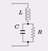 Fig. 8. RLC series circuit with resistance in parallel with the capacitor
A series resistor with the inductor in a parallel LC circuit as shown in figure 7 is a topology commonly encountered where there is a need to take into account the resistance of the coil winding. Parallel LC circuits are frequently used for bandpass filtering and the Q is largely governed by this resistance. The resonant frequency of this circuit is,[17]
This is the resonant frequency of the circuit defined as the frequency at which the admittance has zero imaginary part. The frequency that appears in the generalised form of the characteristic equation (which is the same for this circuit as previously)
is not the same frequency. In this case it is the undamped resonant frequency[18]
The frequency ωm at which the impedance magnitude is maximum is given by,[19]
where
 is the quality factor of the coil. This can be well approximated by,[19]
-
 .
.
Furthermore, the exact maximum impedance magnitude is given by,[19]
-
 .
.
For values of Q greater than unity, this can be well approximated by,[19]
-
 .
.
In the same vein, a resistor in parallel with the capacitor in a series LC circuit can be used to represent a capacitor with a lossy dielectric. This configuration is shown in figure 8. The resonant frequency in this case is given by,[20]
History
The first evidence that a capacitor could produce electrical oscillations was discovered in 1826 by French scientist Felix Savary.[21][22] He found that when a Leyden jar was discharged through a wire wound around an iron needle, sometimes the needle was left magnetized in one direction and sometimes in the opposite direction. He correctly deduced that this was caused by a damped oscillating discharge current in the wire, which reversed the magnetization of the needle back and forth until it was too small to have an effect, leaving the needle magnetized in a random direction.
American physicist Joseph Henry repeated Savary's experiment in 1842 and came to the same conclusion, apparently independently.[23][24] British scientist William Thomson (Lord Kelvin) in 1853 showed mathematically that the discharge of a Leyden jar through an inductance should be oscillatory, and derived its resonant frequency.[23][24][21]
British radio researcher Oliver Lodge, by discharging a large battery of Leyden jars through a long wire, created a tuned circuit with its resonant frequency in the audio range, which produced a musical tone from the spark when it was discharged.[23] In 1857 German physicist Berend Wilhelm Feddersen photographed the spark produced by a resonant Leyden jar circuit in a rotating mirror, providing visible evidence of the oscillations.[23][24][21] In 1868 Scottish physicist James Clerk Maxwell calculated the effect of applying an alternating current to a circuit with inductance and capacitance, showing that the response is maximum at the resonant frequency.[21]
The first example of an electrical resonance curve was published in 1887 by German physicist Heinrich Hertz in his pioneering paper on the discovery of radio waves, showing the length of spark obtainable from his spark-gap LC resonator detectors as a function of frequency.[21]
One of the first demonstrations of resonance between tuned circuits was Lodge's "syntonic jars" experiment around 1889[23][21] He placed two resonant circuits next to each other, each consisting of a Leyden jar connected to an adjustable one-turn coil with a spark gap. When a high voltage from an induction coil was applied to one tuned circuit, creating sparks and thus oscillating currents, sparks were excited in the other tuned circuit only when the inductors were adjusted to resonance. Lodge and some English scientists preferred the term "syntony" for this effect, but the term "resonance" eventually stuck.[21]
The first practical use for RLC circuits was in the 1890s in spark-gap radio transmitters to allow the receiver to be tuned to the transmitter. The first patent for a radio system that allowed tuning was filed by Lodge in 1897, although the first practical systems were invented in 1900 by Anglo Italian radio pioneer Guglielmo Marconi.[21]
Marconi's tuning patents were subsequently overturned in favor of those of Nikola Tesla by the US Supreme Court in December 1943, shortly after Tesla's death.
Applications
Variable tuned circuits
A very frequent use of these circuits is in the tuning circuits of analogue radios. Adjustable tuning is commonly achieved with a parallel plate variable capacitor which allows the value of C to be changed and tune to stations on different frequencies. For the IF stage in the radio where the tuning is preset in the factory the more usual solution is an adjustable core in the inductor to adjust L. In this design the core (made of a high permeability material that has the effect of increasing inductance) is threaded so that it can be screwed further in, or screwed further out of the inductor winding as required.
Filters
 Fig. 9. RLC circuit as a low-pass filter
 Fig. 10. RLC circuit as a high-pass filter
 Fig. 11. RLC circuit as a series band-pass filter in series with the line
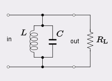 Fig. 12. RLC circuit as a parallel band-pass filter in shunt across the line
 Fig. 13. RLC circuit as a series band-stop filter in shunt across the line
 Fig. 14. RLC circuit as a parallel band-stop filter in series with the line
In the filtering application, the resistor R becomes the load that the filter is working into. The value of the damping factor is chosen based on the desired bandwidth of the filter. For a wider bandwidth, a larger value of the damping factor is required (and vice versa). The three components give the designer three degrees of freedom. Two of these are required to set the bandwidth and resonant frequency. The designer is still left with one which can be used to scale R, L and C to convenient practical values. Alternatively, R may be predetermined by the external circuitry which will use the last degree of freedom.
- Low-pass filter
An RLC circuit can be used as a low-pass filter. The circuit configuration is shown in figure 9. The corner frequency, that is, the frequency of the 3dB point, is given by
This is also the bandwidth of the filter. The damping factor is given by[25]
- High-pass filter
A high-pass filter is shown in figure 10. The corner frequency is the same as the low-pass filter
The filter has a stop-band of this width.[26]
- Band-pass filter
A band-pass filter can be formed with an RLC circuit by either placing a series LC circuit in series with the load resistor or else by placing a parallel LC circuit in parallel with the load resistor. These arrangements are shown in figures 11 and 12 respectively. The centre frequency is given by
and the bandwidth for the series circuit is[27]
The shunt version of the circuit is intended to be driven by a high impedance source, that is, a constant current source. Under those conditions the bandwidth is[27]
- Band-stop filter
Figure 13 shows a band-stop filter formed by a series LC circuit in shunt across the load. Figure 14 is a band-stop filter formed by a parallel LC circuit in series with the load. The first case requires a high impedance source so that the current is diverted into the resonator when it becomes low impedance at resonance. The second case requires a low impedance source so that the voltage is dropped across the antiresonator when it becomes high impedance at resonance.[28]
Oscillators
For applications in oscillator circuits, it is generally desirable to make the attenuation (or equivalently, the damping factor) as small as possible. In practice, this objective requires making the circuit's resistance R as small as physically possible for a series circuit, or alternatively increasing R to as much as possible for a parallel circuit. In either case, the RLC circuit becomes a good approximation to an ideal LC circuit. However, for very low attenuation circuits (high Q-factor) circuits, issues such as dielectric losses of coils and capacitors can become important.
In an oscillator circuit
-
 .
.
or equivalently
-
 .
.
As a result
-
 .
.
Voltage multiplier
In a series RLC circuit at resonance, the current is limited only by the resistance of the circuit
If R is small, consisting only of the inductor winding resistance say, then this current will be large. It will drop a voltage across the inductor of
An equal magnitude voltage will also be seen across the capacitor but in antiphase to the inductor. If R can be made sufficiently small, these voltages can be several times the input voltage. The voltage ratio is, in fact, the Q of the circuit,
A similar effect is observed with currents in the parallel circuit. Even though the circuit appears as high impedance to the external source, there is a large current circulating in the internal loop of the parallel inductor and capacitor.
Pulse discharge circuit
An overdamped series RLC circuit can be used as a pulse discharge circuit. Often it is useful to know the values of components that could be used to produce a waveform this is described by the form:
Such a circuit could consist of an energy storage capacitor, a load in the form of a resistance, some circuit inductance and a switch - all in series. The initial conditions are that the capacitor is at voltage V0 and there is no current flowing in the inductor. If the inductance L is known, then the remaining parameters are given by the following - capacitance:
Resistance (total of circuit and load):
Initial terminal voltage of capacitor:
Rearranging for the case where R is known - Capacitance:
Inductance (total of circuit and load):
Initial terminal voltage of capacitor:
See also
- Bandwidth (signal processing)
- Bandpass filter
- Oliver Heaviside
- Linear circuit
- (3phase circuit)
- [(phasor digrame)]
References
- ^ Kaiser, pp.7.71-7.72.
- ^ Nilsson and Riedel, p.308.
- ^ Agarwal and Lang, p.641.
- ^ Irwin, pp.217-220.
- ^ Agarwal and Lang, p.646.
- ^ a b Agarwal and Lang, p.656.
- ^ Nilsson and Riedel, pp.287-288.
- ^ Irwin, p.532.
- ^ Agarwal and Lang, p.648.
- ^ a b Nilsson and Riedel, p.295.
- ^ Humar, pp.223-224.
- ^ Agarwal and Lang, p.692.
- ^ Nilsson and Riedel, p.303.
- ^ Irwin, p.220.
- ^ This section is based on Example 4.2.13 from Lokenath Debnath, Dambaru Bhatta, Integral transforms and their applications, 2nd ed. Chapman & Hall/CRC, 2007, ISBN 1584885750, pp. 198-202 (some notations have been changed to fit the rest of this article.)
- ^ Nilsson and Riedel, p.286.
- ^ Kaiser, pp.5.26-5.27.
- ^ Agarwal and Lang, p.805.
- ^ a b c d Cartwright, K. V.; Joseph, E. and Kaminsky, E. J. (2010). "Finding the exact maximum impedance resonant frequency of a practical parallel resonant circuit without calculus". The Technology Interface International Journal 11 (1): 26–34. http://www.tiij.org/issues/winter2010/files/TIIJ%20fall-spring%202010-PDW2.pdf.
- ^ Kaiser, pp.5.25-5.26.
- ^ a b c d e f g h Blanchard, Julian (October 1941). "The History of Electrical Resonance". Bell System Technical Journal (USA: American Telephone & Telegraph Co.) 20 (4): 415-. http://www.alcatel-lucent.com/bstj/vol20-1941/articles/bstj20-4-415.pdf. Retrieved 2011-03-29.
- ^ Savary, Felix (1827). "Memoirs sur l'Aimentation". Annales de Chimie et de Physique (Paris: Masson) 34: 5–37.
- ^ a b c d e Kimball, Arthur Lalanne (1917). A College Text-book of Physics, 2nd Ed.. New York: Henry Hold and Co.. pp. 516–517. http://books.google.com/books?id=CwmgAAAAMAAJ&pg=PA516#v=onepage&q&f=false.
- ^ a b c Huurdeman, Anton A. (2003). The worldwide history of telecommunications. USA: Wiley-IEEE. pp. 199–200. ISBN 0471205052. http://books.google.com/books?id=SnjGRDVIUL4C&pg=PA200.
- ^ Kaiser, pp.7.14-7.16.
- ^ Kaiser, p.7.21.
- ^ a b Kaiser, pp.7.21-7.27.
- ^ Kaiser, pp.7.30-7.34.
Bibliography
- Anant Agarwal, Jeffrey H. Lang, Foundations of analog and digital electronic circuits, Morgan Kaufmann, 2005 ISBN 1558607358.
- J. L. Humar, Dynamics of structures, Taylor & Francis, 2002 ISBN 9058092453.
- J. David Irwin, Basic engineering circuit analysis, Wiley, 2006 ISBN 7302130213.
- Kenneth L. Kaiser, Electromagnetic compatibility handbook, CRC Press, 2004 ISBN 0849320879.
- James William Nilsson, Susan A. Riedel, Electric circuits, Prentice Hall, 2008 ISBN 0131989251.
Categories:- Analog circuits
- Electronic filter topology
-


Wikimedia Foundation. 2010.