- Molecular dynamics
-
Molecular dynamics (MD) is a computer simulation of physical movements of atoms and molecules. The atoms and molecules are allowed to interact for a period of time, giving a view of the motion of the atoms. In the most common version, the trajectories of molecules and atoms are determined by numerically solving the Newton's equations of motion for a system of interacting particles, where forces between the particles and potential energy are defined by molecular mechanics force fields. The method was originally conceived within theoretical physics in the late 1950s[1] and early 1960s ,[2] but is applied today mostly in materials science and the modeling of biomolecules.
Because molecular systems consist of a vast number of particles, it is impossible to find the properties of such complex systems analytically; MD simulation circumvents this problem by using numerical methods. However, long MD simulations are mathematically ill-conditioned, generating cumulative errors in numerical integration that can be minimized with proper selection of algorithms and parameters, but not eliminated entirely.
The results of molecular dynamics simulations may be used to determine macroscopic thermodynamic properties of the system based on the ergodic hypothesis: the statistical ensemble averages are equal to time averages of the system. MD has also been termed "statistical mechanics by numbers" and "Laplace's vision of Newtonian mechanics" of predicting the future by animating nature's forces[3][4] and allowing insight into molecular motion on an atomic scale.
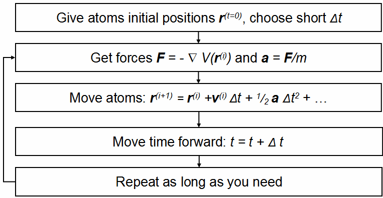
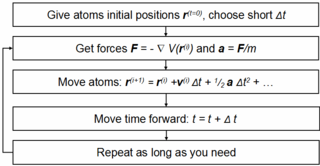 Highly simplified description of the molecular dynamics simulation algorithm. The simulation proceeds iteratively by alternatively calculating forces and solving the equations of motion based on the accelerations obtained from the new forces. In practise, almost all MD codes use much more complicated versions of the algorithm, including two steps (predictor and corrector) in solving the equations of motion and many additional steps for e.g. temperature and pressure control, analysis and output.
Contents
History
Before it became possible to simulate molecular dynamics with computers, some undertook the hard work of trying it with physical models such as macroscopic spheres. The idea was to arrange them to replicate the properties of a liquid. J.D. Bernal said, in 1962: "... I took a number of rubber balls and stuck them together with rods of a selection of different lengths ranging from 2.75 to 4 inches. I tried to do this in the first place as casually as possible, working in my own office, being interrupted every five minutes or so and not remembering what I had done before the interruption."[5] Fortunately, now computers keep track of bonds during a simulation.
Areas of Application
There is a significant difference between the focus and methods used by chemists and physicists, and this is reflected in differences in the jargon used by the different fields. In chemistry and biophysics, the interaction between the particles is either described by a "force field" (classical MD), a quantum chemical model, or a mix between the two. These terms are not used in physics, where the interactions are usually described by the name of the theory or approximation being used and called the potential energy, or just the "potential".
Beginning in theoretical physics, the method of MD gained popularity in materials science and since the 1970s also in biochemistry and biophysics. In chemistry, MD serves as an important tool in protein structure determination and refinement using experimental tools such as X-ray crystallography and NMR. It has also been applied with limited success as a method of refining protein structure predictions. In physics, MD is used to examine the dynamics of atomic-level phenomena that cannot be observed directly, such as thin film growth and ion-subplantation. It is also used to examine the physical properties of nanotechnological devices that have not or cannot yet be created.
In applied mathematics and theoretical physics, molecular dynamics is a part of the research realm of dynamical systems, ergodic theory and statistical mechanics in general. The concepts of energy conservation and molecular entropy come from thermodynamics. Some techniques to calculate conformational entropy such as principal components analysis come from information theory. Mathematical techniques such as the transfer operator become applicable when MD is seen as a Markov chain. Also, there is a large community of mathematicians working on volume preserving, symplectic integrators for more computationally efficient MD simulations.
MD can also be seen as a special case of the discrete element method (DEM) in which the particles have spherical shape (e.g. with the size of their van der Waals radii.) Some authors in the DEM community employ the term MD rather loosely, even when their simulations do not model actual molecules.
Steered Molecular Dynamics (SMD)
Steered molecular dynamics (SMD) simulations, or Force Probe Simulations, apply forces to a protein in order to manipulate its structure by pulling it along desired degrees of freedom. These experiments can be used to reveal structural changes in a protein at the atomic level. SMD is often used to simulate events such as mechanical unfolding or stretching.[6]
There are two typical protocols of SMD: one in which pulling velocity is held constant and one in which applied force is constant. Typically, part of the studied system (eg. An atom in a protein) is restrained by a harmonic potential. Forces are then applied to specific atoms at either a constant velocity or a constant force. Umbrella Sampling is used to move the system along the desired reaction coordinate by varying, for example, the forces, distances, and angles manipulated in the simulation. Through umbrella sampling, all of the system's configurations—both high-energy and low-energy—are adequately sampled. Then, each configuration's change in free energy can be calculated as the potential mean force.[7] A popular method of computing PMF is through the weighted histogram analysis method (WHAM), which analyzes a series of umbrella sampling simulations.[8]
Design Constraints
Design of a molecular dynamics simulation should account for the available computational power. Simulation size (n=number of particles), timestep and total time duration must be selected so that the calculation can finish within a reasonable time period. However, the simulations should be long enough to be relevant to the time scales of the natural processes being studied. To make statistically valid conclusions from the simulations, the time span simulated should match the kinetics of the natural process. Otherwise, it is analogous to making conclusions about how a human walks from less than one footstep. Most scientific publications about the dynamics of proteins and DNA use data from simulations spanning nanoseconds (10−9 s) to microseconds (10−6 s). To obtain these simulations, several CPU-days to CPU-years are needed. Parallel algorithms allow the load to be distributed among CPUs; an example is the spatial or force decomposition algorithm [1].
During a classical MD simulation, the most CPU intensive task is the evaluation of the potential (force field) as a function of the particles' internal coordinates. Within that energy evaluation, the most expensive one is the non-bonded or non-covalent part. In Big O notation, common molecular dynamics simulations scale by O(n2) if all pair-wise electrostatic and van der Waals interactions must be accounted for explicitly. This computational cost can be reduced by employing electrostatics methods such as Particle Mesh Ewald ( O(nlog(n)) ), P3M or good spherical cutoff techniques ( O(n) ).
Another factor that impacts total CPU time required by a simulation is the size of the integration timestep. This is the time length between evaluations of the potential. The timestep must be chosen small enough to avoid discretization errors (i.e. smaller than the fastest vibrational frequency in the system). Typical timesteps for classical MD are in the order of 1 femtosecond (10−15 s). This value may be extended by using algorithms such as SHAKE, which fix the vibrations of the fastest atoms (e.g. hydrogens) into place. Multiple time scale methods have also been developed, which allow for extended times between updates of slower long-range forces.[9][10][11]
For simulating molecules in a solvent, a choice should be made between explicit solvent and implicit solvent. Explicit solvent particles (such as the TIP3P, SPC/E and SPC-f water models) must be calculated expensively by the force field, while implicit solvents use a mean-field approach. Using an explicit solvent is computationally expensive, requiring inclusion of roughly ten times more particles in the simulation. But the granularity and viscosity of explicit solvent is essential to reproduce certain properties of the solute molecules. This is especially important to reproduce kinetics.
In all kinds of molecular dynamics simulations, the simulation box size must be large enough to avoid boundary condition artifacts. Boundary conditions are often treated by choosing fixed values at the edges (which may cause artifacts), or by employing periodic boundary conditions in which one side of the simulation loops back to the opposite side, mimicking a bulk phase.
Microcanonical ensemble (NVE)
In the microcanonical, or NVE ensemble, the system is isolated from changes in moles (N), volume (V) and energy (E). It corresponds to an adiabatic process with no heat exchange. A microcanonical molecular dynamics trajectory may be seen as an exchange of potential and kinetic energy, with total energy being conserved. For a system of N particles with coordinates X and velocities V, the following pair of first order differential equations may be written in Newton's notation as
The potential energy function U(X) of the system is a function of the particle coordinates X. It is referred to simply as the "potential" in Physics, or the "force field" in Chemistry. The first equation comes from Newton's laws; the force F acting on each particle in the system can be calculated as the negative gradient of U(X).
For every timestep, each particle's position X and velocity V may be integrated with a symplectic method such as Verlet. The time evolution of X and V is called a trajectory. Given the initial positions (e.g. from theoretical knowledge) and velocities (e.g. randomized Gaussian), we can calculate all future (or past) positions and velocities.
One frequent source of confusion is the meaning of temperature in MD. Commonly we have experience with macroscopic temperatures, which involve a huge number of particles. But temperature is a statistical quantity. If there is a large enough number of atoms, statistical temperature can be estimated from the instantaneous temperature, which is found by equating the kinetic energy of the system to nkBT/2 where n is the number of degrees of freedom of the system.
A temperature-related phenomenon arises due to the small number of atoms that are used in MD simulations. For example, consider simulating the growth of a copper film starting with a substrate containing 500 atoms and a deposition energy of 100 eV. In the real world, the 100 eV from the deposited atom would rapidly be transported through and shared among a large number of atoms (1010 or more) with no big change in temperature. When there are only 500 atoms, however, the substrate is almost immediately vaporized by the deposition. Something similar happens in biophysical simulations. The temperature of the system in NVE is naturally raised when macromolecules such as proteins undergo exothermic conformational changes and binding.
Canonical ensemble (NVT)
In the canonical ensemble, moles (N), volume (V) and temperature (T) are conserved. It is also sometimes called constant temperature molecular dynamics (CTMD). In NVT, the energy of endothermic and exothermic processes is exchanged with a thermostat.
A variety of thermostat methods is available to add and remove energy from the boundaries of an MD system in a more or less realistic way, approximating the canonical ensemble. Popular techniques to control temperature include velocity rescaling, the Nosé-Hoover thermostat, Nosé-Hoover chains, the Berendsen thermostat and Langevin dynamics. Note that the Berendsen thermostat might introduce the flying ice cube effect, which leads to unphysical translations and rotations of the simulated system.
It is not trivial to obtain a canonical distribution of conformations and velocities using these algorithms. How this depends on system size, thermostat choice, thermostat parameters, time step and integrator is the subject of many articles in the field.
Isothermal-Isobaric (NPT) ensemble
In the isothermal-isobaric ensemble, moles (N), pressure (P) and temperature (T) are conserved. In addition to a thermostat, a barostat is needed. It corresponds most closely to laboratory conditions with a flask open to ambient temperature and pressure.
In the simulation of biological membranes, isotropic pressure control is not appropriate. For lipid bilayers, pressure control occurs under constant membrane area (NPAT) or constant surface tension "gamma" (NPγT).
Generalized ensembles
The replica exchange method is a generalized ensemble. It was originally created to deal with the slow dynamics of disordered spin systems. It is also called parallel tempering. The replica exchange MD (REMD) formulation [12] tries to overcome the multiple-minima problem by exchanging the temperature of non-interacting replicas of the system running at several temperatures.
Potentials in MD simulations
Main articles: Force field and Force field implementationA molecular dynamics simulation requires the definition of a potential function, or a description of the terms by which the particles in the simulation will interact. In chemistry and biology this is usually referred to as a force field. Potentials may be defined at many levels of physical accuracy; those most commonly used in chemistry are based on molecular mechanics and embody a classical treatment of particle-particle interactions that can reproduce structural and conformational changes but usually cannot reproduce chemical reactions.
The reduction from a fully quantum description to a classical potential entails two main approximations. The first one is the Born-Oppenheimer approximation, which states that the dynamics of electrons is so fast that they can be considered to react instantaneously to the motion of their nuclei. As a consequence, they may be treated separately. The second one treats the nuclei, which are much heavier than electrons, as point particles that follow classical Newtonian dynamics. In classical molecular dynamics the effect of the electrons is approximated as a single potential energy surface, usually representing the ground state.
When finer levels of detail are required, potentials based on quantum mechanics are used; some techniques attempt to create hybrid classical/quantum potentials where the bulk of the system is treated classically but a small region is treated as a quantum system, usually undergoing a chemical transformation.
Empirical potentials
Empirical potentials used in chemistry are frequently called force fields, while those used in materials physics are called just empirical or analytical potentials.
Most force fields in chemistry are empirical and consist of a summation of bonded forces associated with chemical bonds, bond angles, and bond dihedrals, and non-bonded forces associated with van der Waals forces and electrostatic charge. Empirical potentials represent quantum-mechanical effects in a limited way through ad-hoc functional approximations. These potentials contain free parameters such as atomic charge, van der Waals parameters reflecting estimates of atomic radius, and equilibrium bond length, angle, and dihedral; these are obtained by fitting against detailed electronic calculations (quantum chemical simulations) or experimental physical properties such as elastic constants, lattice parameters and spectroscopic measurements.
Because of the non-local nature of non-bonded interactions, they involve at least weak interactions between all particles in the system. Its calculation is normally the bottleneck in the speed of MD simulations. To lower the computational cost, force fields employ numerical approximations such as shifted cutoff radii, reaction field algorithms, particle mesh Ewald summation, or the newer Particle-Particle Particle Mesh (P3M).
Chemistry force fields commonly employ preset bonding arrangements (an exception being ab-initio dynamics), and thus are unable to model the process of chemical bond breaking and reactions explicitly. On the other hand, many of the potentials used in physics, such as those based on the bond order formalism can describe several different coordinations of a system and bond breaking. Examples of such potentials include the Brenner potential[13] for hydrocarbons and its further developments for the C-Si-H and C-O-H systems. The ReaxFF potential[14] can be considered a fully reactive hybrid between bond order potentials and chemistry force fields.
Pair potentials vs. many-body potentials
The potential functions representing the non-bonded energy are formulated as a sum over interactions between the particles of the system. The simplest choice, employed in many popular force field (physics), is the "pair potential", in which the total potential energy can be calculated from the sum of energy contributions between pairs of atoms. An example of such a pair potential is the non-bonded Lennard-Jones potential (also known as the 6-12 potential), used for calculating van der Waals forces.
Another example is the Born (ionic) model of the ionic lattice. The first term in the next equation is Coulomb's law for a pair of ions, the second term is the short-range repulsion explained by Pauli's exclusion principle and the final term is the dispersion interaction term. Usually, a simulation only includes the dipolar term, although sometimes the quadrupolar term is included as well.
In many-body potentials, the potential energy includes the effects of three or more particles interacting with each other. In simulations with pairwise potentials, global interactions in the system also exist, but they occur only through pairwise terms. In many-body potentials, the potential energy cannot be found by a sum over pairs of atoms, as these interactions are calculated explicitly as a combination of higher-order terms. In the statistical view, the dependency between the variables cannot in general be expressed using only pairwise products of the degrees of freedom. For example, the Tersoff potential,[15] which was originally used to simulate carbon, silicon and germanium and has since been used for a wide range of other materials, involves a sum over groups of three atoms, with the angles between the atoms being an important factor in the potential. Other examples are the embedded-atom method (EAM)[16] and the Tight-Binding Second Moment Approximation (TBSMA) potentials,[17] where the electron density of states in the region of an atom is calculated from a sum of contributions from surrounding atoms, and the potential energy contribution is then a function of this sum.
Semi-empirical potentials
Semi-empirical potentials make use of the matrix representation from quantum mechanics. However, the values of the matrix elements are found through empirical formulae that estimate the degree of overlap of specific atomic orbitals. The matrix is then diagonalized to determine the occupancy of the different atomic orbitals, and empirical formulae are used once again to determine the energy contributions of the orbitals.
There are a wide variety of semi-empirical potentials, known as tight-binding potentials, which vary according to the atoms being modeled.
Polarizable potentials
Main article: Force fieldMost classical force fields implicitly include the effect of polarizability, e.g. by scaling up the partial charges obtained from quantum chemical calculations. These partial charges are stationary with respect to the mass of the atom. But molecular dynamics simulations can explicitly model polarizability with the introduction of induced dipoles through different methods, such as Drude particles or fluctuating charges. This allows for a dynamic redistribution of charge between atoms which responds to the local chemical environment.
For many years, polarizable MD simulations have been touted as the next generation. For homogenous liquids such as water, increased accuracy has been achieved through the inclusion of polarizability.[18] Some promising results have also been achieved for proteins.[19] However, it is still uncertain how to best approximate polarizability in a simulation.[citation needed]
Ab-initio methods
In classical molecular dynamics, a single potential energy surface (usually the ground state) is represented in the force field. This is a consequence of the Born-Oppenheimer approximation. In excited states, chemical reactions or when a more accurate representation is needed, electronic behavior can be obtained from first principles by using a quantum mechanical method, such as Density Functional Theory. This is known as Ab Initio Molecular Dynamics (AIMD). Due to the cost of treating the electronic degrees of freedom, the computational cost of this simulations is much higher than classical molecular dynamics. This implies that AIMD is limited to smaller systems and shorter periods of time.
Ab-initio quantum-mechanical methods may be used to calculate the potential energy of a system on the fly, as needed for conformations in a trajectory. This calculation is usually made in the close neighborhood of the reaction coordinate. Although various approximations may be used, these are based on theoretical considerations, not on empirical fitting. Ab-Initio calculations produce a vast amount of information that is not available from empirical methods, such as density of electronic states or other electronic properties. A significant advantage of using ab-initio methods is the ability to study reactions that involve breaking or formation of covalent bonds, which correspond to multiple electronic states.
A popular software for ab-initio molecular dynamics is the Car-Parrinello Molecular Dynamics (CPMD) package based on the density functional theory.
Hybrid QM/MM
QM (quantum-mechanical) methods are very powerful. However, they are computationally expensive, while the MM (classical or molecular mechanics) methods are fast but suffer from several limitations (require extensive parameterization; energy estimates obtained are not very accurate; cannot be used to simulate reactions where covalent bonds are broken/formed; and are limited in their abilities for providing accurate details regarding the chemical environment). A new class of method has emerged that combines the good points of QM (accuracy) and MM (speed) calculations. These methods are known as mixed or hybrid quantum-mechanical and molecular mechanics methods (hybrid QM/MM).[20]
The most important advantage of hybrid QM/MM methods is the speed. The cost of doing classical molecular dynamics (MM) in the most straightforward case scales O(n2), where n is the number of atoms in the system. This is mainly due to electrostatic interactions term (every particle interacts with every other particle). However, use of cutoff radius, periodic pair-list updates and more recently the variations of the particle-mesh Ewald's (PME) method has reduced this between O(n) to O(n2). In other words, if a system with twice as many atoms is simulated then it would take between two to four times as much computing power. On the other hand the simplest ab-initio calculations typically scale O(n3) or worse (Restricted Hartree-Fock calculations have been suggested to scale ~O(n2.7)). To overcome the limitation, a small part of the system is treated quantum-mechanically (typically active-site of an enzyme) and the remaining system is treated classically.
In more sophisticated implementations, QM/MM methods exist to treat both light nuclei susceptible to quantum effects (such as hydrogens) and electronic states. This allows generation of hydrogen wave-functions (similar to electronic wave-functions). This methodology has been useful in investigating phenomena such as hydrogen tunneling. One example where QM/MM methods have provided new discoveries is the calculation of hydride transfer in the enzyme liver alcohol dehydrogenase. In this case, tunneling is important for the hydrogen, as it determines the reaction rate.[21]
Coarse-graining and reduced representations
At the other end of the detail scale are coarse-grained and lattice models. Instead of explicitly representing every atom of the system, one uses "pseudo-atoms" to represent groups of atoms. MD simulations on very large systems may require such large computer resources that they cannot easily be studied by traditional all-atom methods. Similarly, simulations of processes on long timescales (beyond about 1 microsecond) are prohibitively expensive, because they require so many timesteps. In these cases, one can sometimes tackle the problem by using reduced representations, which are also called coarse-grained models.
Examples for coarse graining (CG) methods are discontinuous molecular dynamics (CG-DMD)[22][23] and Go-models.[24] Coarse-graining is done sometimes taking larger pseudo-atoms. Such united atom approximations have been used in MD simulations of biological membranes. The aliphatic tails of lipids are represented by a few pseudo-atoms by gathering 2 to 4 methylene groups into each pseudo-atom.
The parameterization of these very coarse-grained models must be done empirically, by matching the behavior of the model to appropriate experimental data or all-atom simulations. Ideally, these parameters should account for both enthalpic and entropic contributions to free energy in an implicit way. When coarse-graining is done at higher levels, the accuracy of the dynamic description may be less reliable. But very coarse-grained models have been used successfully to examine a wide range of questions in structural biology, liquid crystal organization, and polymer glasses.
Examples of applications of coarse-graining:
- protein folding studies are often carried out using a single (or a few) pseudo-atoms per amino acid;
- liquid crystal phase transitions have been examined in confined geometries and/or during flow using the Gay-Berne potential which describes anisotropic species;
- Polymer glasses during deformation have been studied using simple harmonic or FENE springs to connect spheres described by the Lennard-Jones potential;
- DNA supercoiling has been investigated using 1-3 pseudo-atoms per basepair, and at even lower resolution;
- Packaging of double-helical DNA into bacteriophage has been investigated with models where one pseudo-atom represents one turn (about 10 basepairs) of the double helix;
- RNA structure in the ribosome and other large systems has been modeled with one pseudo-atom per nucleotide.
The simplest form of coarse-graining is the "united atom" (sometimes called "extended atom") and was used in most early MD simulations of proteins, lipids and nucleic acids. For example, instead of treating all four atoms of a CH3 methyl group explicitly (or all three atoms of CH2 methylene group), one represents the whole group with a single pseudo-atom. This pseudo-atom must, of course, be properly parameterized so that its van der Waals interactions with other groups have the proper distance-dependence. Similar considerations apply to the bonds, angles, and torsions in which the pseudo-atom participates. In this kind of united atom representation, one typically eliminates all explicit hydrogen atoms except those that have the capability to participate in hydrogen bonds ("polar hydrogens"). An example of this is the Charmm 19 force-field.
The polar hydrogens are usually retained in the model, because proper treatment of hydrogen bonds requires a reasonably accurate description of the directionality and the electrostatic interactions between the donor and acceptor groups. A hydroxyl group, for example, can be both a hydrogen bond donor and a hydrogen bond acceptor, and it would be impossible to treat this with a single OH pseudo-atom. Note that about half the atoms in a protein or nucleic acid are nonpolar hydrogens, so the use of united atoms can provide a substantial savings in computer time.
Examples of applications
Molecular dynamics is used in many fields of science.
- First macromolecular MD simulation published (1977, Size: 500 atoms, Simulation Time: 9.2 ps=0.0092 ns, Program: CHARMM precursor) Protein: Bovine Pancreatic Trypsine Inhibitor. This is one of the best studied proteins in terms of folding and kinetics. Its simulation published in Nature magazine paved the way for understanding protein motion as essential in function and not just accessory.[25]
- MD is the standard method to treat collision cascades in the heat spike regime, i.e. the effects that energetic neutron and ion irradiation have on solids an solid surfaces.[26][27]
- MD simulations were successfully applied to predict the molecular basis of the most common protein mutation N370S, causing Gaucher Disease[28]. In a follow-up publication it was shown that these blind predictions show a surprisingly high correlation with experimental work on the same mutant, published independently at a later point[29].
The following two biophysical examples are not run-of-the-mill MD simulations. They illustrate notable efforts to produce simulations of a system of very large size (a complete virus) and very long simulation times (500 microseconds):
- MD simulation of the complete satellite tobacco mosaic virus (STMV) (2006, Size: 1 million atoms, Simulation time: 50 ns, program: NAMD) This virus is a small, icosahedral plant virus which worsens the symptoms of infection by Tobacco Mosaic Virus (TMV). Molecular dynamics simulations were used to probe the mechanisms of viral assembly. The entire STMV particle consists of 60 identical copies of a single protein that make up the viral capsid (coating), and a 1063 nucleotide single stranded RNA genome. One key finding is that the capsid is very unstable when there is no RNA inside. The simulation would take a single 2006 desktop computer around 35 years to complete. It was thus done in many processors in parallel with continuous communication between them.[30]
- Folding Simulations of the Villin Headpiece in All-Atom Detail (2006, Size: 20,000 atoms; Simulation time: 500 µs = 500,000 ns, Program: Folding@home) This simulation was run in 200,000 CPU's of participating personal computers around the world. These computers had the Folding@home program installed, a large-scale distributed computing effort coordinated by Vijay Pande at Stanford University. The kinetic properties of the Villin Headpiece protein were probed by using many independent, short trajectories run by CPU's without continuous real-time communication. One technique employed was the Pfold value analysis, which measures the probability of folding before unfolding of a specific starting conformation. Pfold gives information about transition state structures and an ordering of conformations along the folding pathway. Each trajectory in a Pfold calculation can be relatively short, but many independent trajectories are needed.[31]
Molecular dynamics algorithms
Integrators
- Verlet-Stoermer integration
- Runge-Kutta integration
- Beeman's algorithm
- Constraint algorithms (for constrained systems)
- Symplectic integrator
Short-range interaction algorithms
- Cell lists
- Verlet list
- Bonded interactions
Long-range interaction algorithms
- Ewald summation
- Particle Mesh Ewald (PME)
- Particle-Particle Particle Mesh P3M
Parallelization strategies
- Domain decomposition method (Distribution of system data for parallel computing)
Major software for MD simulations
Main article: List of software for molecular mechanics modeling- AutoDock suite of automated docking tools,
- Abalone (classical, implicit water, GPU accelerated)
- ABINIT (DFT)
- ACEMD (classical), GPU accelerated)
- AMBER (classical ,GPU accelerated)
- Ascalaph Designer (classical)
- CASTEP (DFT)
- CP2K (DFT)
- CPMD (DFT)
- CHARMM (classical, the pioneer in MD simulation, extensive analysis tools)
- Desmond (classical, parallelization with up to thousands of CPU's)
- GPAW (DFT, large-scale parallelisation) See https://wiki.fysik.dtu.dk/gpaw/
- GPIUTMD (classical, GPU accelerated)
- GROMACS (classical, GPU accelerated)
- GROMOS (classical)
- HOOMD-blue (classical, GPU accelerated)
- LAMMPS (classical, large-scale with spatial-decomposition of simulation domain for parallelism)
- LPMD (classical, with many additional utilities)
- MacroModel (classical)
- MDynaMix (classical, parallel)
- MOSCITO (classical)
- NAMD (classical, parallelization with up to thousands of CPU's, GPU accelerated)
- ORAC (classical)
- PWscf (DFT)
- SIESTA (DFT)
- Tremolo-X (classical, parallelization with up to thousands of CPU's)
- VASP (DFT)
- TINKER (classical)
- XMD (classical)
Related software
- Avizo - 3d visualization and analysis software.
- BOSS - MC in OPLS
- Chimera - Molecular visualization and analysis package, including trajectory support.
- PyMol - Molecular Visualization software written in python.
- Sirius - Molecular modeling, analysis and visualization of MD trajectories.
- VMD - MD simulation trajectories can be visualized and analyzed.
- Folding@Home - A distributed computing project to study protein folding.
Specialized hardware for MD simulations
- Anton - A specialized, massively parallel supercomputer designed to execute MD simulations.
- MDGRAPE - A special purpose system built for molecular dynamics simulations, especially protein structure prediction.
See also
- Molecule editor
- Molecular graphics
- Molecular modeling
- Computational chemistry
- Energy drift
- Force field (chemistry)
- Force field implementation
- Monte Carlo method
- Molecular design software
- Molecular mechanics
- Molecular modeling on GPU
- Protein dynamics
- Implicit solvation
- Car-Parrinello method
- Symplectic numerical integration
- Software for molecular mechanics modeling
- List of software for Monte Carlo molecular modeling
- Dynamical systems
- Theoretical chemistry
- Statistical mechanics
- Quantum chemistry
- Discrete element method
- List of nucleic acid simulation software
- List of molecular graphics systems
- List of web resources for visualizing molecular dynamics
References
- ^ Alder, B. J.; T. E. Wainwright (1959). "Studies in Molecular Dynamics. I. General Method". J. Chem. Phys. 31 (2): 459. Bibcode 1959JChPh..31..459A. doi:10.1063/1.1730376.
- ^ A. Rahman (1964). "Correlations in the Motion of Atoms in Liquid Argon". Phys Rev 136 (2A): A405-A411. Bibcode 1964PhRv..136..405R. doi:10.1103/PhysRev.136.A405.
- ^ Schlick, T. (1996). "Pursuing Laplace's Vision on Modern Computers". In J. P. Mesirov, K. Schulten and D. W. Sumners. Mathematical Applications to Biomolecular Structure and Dynamics, IMA Volumes in Mathematics and Its Applications. 82. New York: Springer-Verlag. pp. 218–247. ISBN 978-0387948386.
- ^ de Laplace, P. S. (1820) (in French). Oeuveres Completes de Laplace, Theorie Analytique des Probabilites. Paris, France: Gauthier-Villars.
- ^ Bernal, J.D. (1964). "The Bakerian lecture, 1962: The structure of liquids". Proc. R. Soc. 280 (1382): 299–322. Bibcode 1964RSPSA.280..299B. doi:10.1098/rspa.1964.0147.
- ^ Nienhaus, Gerd Ulrich (2005). Protein-ligand interactions: methods and applications. pp. 54–56. ISBN 978-1617375255.
- ^ Leszczynski, Jerzy (2005). Computational chemistry: reviews of current trends, Volume 9. pp. 54–56. ISBN 978-9812567420.
- ^ Kumar, Shankar; Rosenberg, John M., Bouzida, Djamal, Swendsen, Robert H., Kollman, Peter A. (30 September 1992). "THE weighted histogram analysis method for free-energy calculations on biomolecules. I. The method". Journal of Computational Chemistry 13 (8): 1011–1021. doi:10.1002/jcc.540130812.
- ^ Streett WB, Tildesley DJ, Saville G (1978). "Multiple time-step methods in molecular dynamics". Mol Phys 35 (3): 639–648. Bibcode 1978MolPh..35..639S. doi:10.1080/00268977800100471.
- ^ Tuckerman ME, Berne BJ, Martyna GJ (1991). "Molecular dynamics algorithm for multiple time scales: systems with long range forces". J Chem Phys 94 (10): 6811–6815. Bibcode 1991JChPh..94.6811T. doi:10.1063/1.460259.
- ^ Tuckerman ME, Berne BJ, Martyna GJ (1992). "Reversible multiple time scale molecular dynamics". J Chem Phys 97 (3): 1990–2001. Bibcode 1992JChPh..97.1990T. doi:10.1063/1.463137.
- ^ Sugita, Yuji; Yuko Okamoto (1999). "Replica-exchange molecular dynamics method for protein folding". Chem Phys Letters 314: 141–151. Bibcode 1999CPL...314..141S. doi:10.1016/S0009-2614(99)01123-9.
- ^ Brenner, D. W. (1990). "Empirical potential for hydrocarbons for use in simulating the chemical vapor deposition of diamond films". Phys. Rev. B 42 (15): 9458. Bibcode 1990PhRvB..42.9458B. doi:10.1103/PhysRevB.42.9458.
- ^ van Duin, A.; Siddharth Dasgupta, Francois Lorant and William A. Goddard III (2001). J. Phys. Chem. A 105: 9398.
- ^ Tersoff, J. (1989). "Modeling solid-state chemistry: Interatomic potentials for multicomponent systems". Phys. Rev. B 39 (8): 5566. Bibcode 1989PhRvB..39.5566T. doi:10.1103/PhysRevB.39.5566.
- ^ Daw, M. S.; S. M. Foiles and M. I. Baskes (1993). "The embedded-atom method: a review of theory and applications". Mat. Sci. And Engr. Rep. 9 (7-8): 251. doi:10.1016/0920-2307(93)90001-U.
- ^ Cleri, F.; V. Rosato (1993). "Tight-binding potentials for transition metals and alloys". Phys. Rev. B 48: 22. Bibcode 1993PhRvB..48...22C. doi:10.1103/PhysRevB.48.22.
- ^ Lamoureux G, Harder E, Vorobyov IV, Roux B, MacKerell AD (2006). "A polarizable model of water for molecular dynamics simulations of biomolecules". Chem Phys Lett 418: 245–249. Bibcode 2006CPL...418..245L. doi:10.1016/j.cplett.2005.10.135.
- ^ Patel, S.; MacKerell, Jr. AD; Brooks III, Charles L (2004). "CHARMM fluctuating charge force field for proteins: II protein/solvent properties from molecular dynamics simulations using a nonadditive electrostatic model". J Comput Chem 25 (12): 1504–1514. doi:10.1002/jcc.20077. PMID 15224394.
- ^ The methodology for such techniques was introduced by Warshel and coworkers. In the recent years have been pioneered by several groups including: Arieh Warshel (University of Southern California), Weitao Yang (Duke University), Sharon Hammes-Schiffer (The Pennsylvania State University), Donald Truhlar and Jiali Gao (University of Minnesota) and Kenneth Merz (University of Florida).
- ^ Billeter, SR; SP Webb, PK Agarwal, T Iordanov, S Hammes-Schiffer (2001). "Hydride Transfer in Liver Alcohol Dehydrogenase: Quantum Dynamics, Kinetic Isotope Effects, and Role of Enzyme Motion". J Am Chem Soc 123 (45): 11262–11272. doi:10.1021/ja011384b. PMID 11697969.
- ^ Smith, A; CK Hall (2001). "Alpha-Helix Formation: Discontinuous Molecular Dynamics on an Intermediate-Resolution Protein Model". Proteins 44 (3): 344–360. doi:10.1002/prot.1100. PMID 11455608.
- ^ Ding, F; JM Borreguero, SV Buldyrey, HE Stanley, NV Dokholyan (2003). "Mechanism for the alpha-helix to beta-hairpin transition". J Am Chem Soc 53 (2): 220–228. doi:10.1002/prot.10468. PMID 14517973.
- ^ Paci, E; M Vendruscolo, M Karplus (2002). "Validity of Go Models: Comparison with a Solvent-Shielded Empirical Energy Decomposition". Biophys J 83 (6): 3032–3038. Bibcode 2002BpJ....83.3032P. doi:10.1016/S0006-3495(02)75308-3. PMC 1302383. PMID 12496075. http://www.pubmedcentral.nih.gov/articlerender.fcgi?tool=pmcentrez&artid=1302383.
- ^ McCammon, J; JB Gelin, M Karplus (1977). "Dynamics of folded proteins". Nature 267 (5612): 585–590. Bibcode 1977Natur.267..585M. doi:10.1038/267585a0. PMID 301613.
- ^ Averback, R. S.; Diaz de la Rubia, T. (1998). "Displacement damage in irradiated metals and semiconductors". In H. Ehrenfest and F. Spaepen. Solid State Physics. 51. New York: Academic Press. pp. 281–402.
- ^ R. Smith, ed (1997). Atomic & ion collisions in solids and at surfaces: theory, simulation and applications. Cambridge, UK: Cambridge University Press.
- ^ Offman, MN; M Krol, I Silman, JL Sussman, AH Futerman (2010). "Molecular basis of reduced glucosylceramidase activity in the most common Gaucher disease mutant, N370S". J. Biol. Chem. 285: 42105-42114. PMID 20980259.
- ^ Offman, MN; M Krol, B Rost, I Silman, JL Sussman, AH Futerman (2011). "Comparison of a molecular dynamics model with the X-ray structure of the N370S acid-beta-glucosidase mutant that causes Gaucher disease". Protein Eng. Des. Sel. 24: 773-775. PMID 21724649.
- ^ Freddolino P, Arkhipov A, Larson SB, McPherson A, Schulten K. "Molecular dynamics simulation of the Satellite Tobacco Mosaic Virus (STMV)". Theoretical and Computational Biophysics Group. University of Illinois at Urbana Champaign. http://www.ks.uiuc.edu/Research/STMV/.
- ^ The Folding@Home Project and recent papers published using trajectories from it. Vijay Pande Group. Stanford University
General references
- M. P. Allen, D. J. Tildesley (1989) Computer simulation of liquids. Oxford University Press. ISBN 0-19-855645-4.
- J. A. McCammon, S. C. Harvey (1987) Dynamics of Proteins and Nucleic Acids. Cambridge University Press. ISBN 0521307503 (hardback).
- D. C. Rapaport (1996) The Art of Molecular Dynamics Simulation. ISBN 0-521-44561-2.
- M. Griebel, S. Knapek, G. Zumbusch: Numerical Simulation in Molecular Dynamics. Springer, Berlin, Heidelberg 2 November 2011, ISBN 978-3-540-68094-9.
- Frenkel, Daan; Smit, Berend (2002) [2001]. Understanding Molecular Simulation : from algorithms to applications. San Diego, California: Academic Press. ISBN 0-12-267351-4.
- J. M. Haile (2001) Molecular Dynamics Simulation: Elementary Methods. ISBN 0-471-18439-X
- R. J. Sadus, Molecular Simulation of Fluids: Theory, Algorithms and Object-Orientation, 2002, ISBN 0-444-51082-6
- Oren M. Becker, Alexander D. Mackerell Jr, Benoît Roux, Masakatsu Watanabe (2001) Computational Biochemistry and Biophysics. Marcel Dekker. ISBN 0-8247-0455-X.
- Andrew Leach (2001) Molecular Modelling: Principles and Applications. (2nd Edition) Prentice Hall. ISBN 978-0582382107.
- Tamar Schlick (2002) Molecular Modeling and Simulation. Springer. ISBN 0-387-95404-X.
- William Graham Hoover (1991) Computational Statistical Mechanics, Elsevier, ISBN 0-444-88192-1.
- D.J. Evans and G.P. Morriss (2008) Statistical Mechanics of Nonequilibrium Liquids, Second Edition, Cambridge University Press,ISBN 978-0-521-85791-8.
External links
- The GPUGRID.net Project (GPUGRID.net)
- The Blue Gene Project (IBM)JawBreakers.org
- D. E. Shaw Research (D. E. Shaw Research)
- Molecular Physics
- Statistical mechanics of Nonequilibrium Liquids Lecture Notes on non-equilibrium MD
- Introductory Lecture on Classical Molecular Dynamics by Dr. Godehard Sutmann, NIC, Forschungszentrum Jülich, Germany
- Introductory Lecture on Ab Initio Molecular Dynamics and Ab Initio Path Integrals by Mark E. Tuckerman, New York University, USA
- Introductory Lecture on Ab initio molecular dynamics: Theory and Implementation by Dominik Marx, Ruhr-Universität Bochum and Jürg Hutter, Universität Zürich
- Online course on (MSE 597G) An Introduction to Molecular Dynamics by Alejandro Strachan
- Lecture Notes on Short Course on Molecular Dynamics Simulation Ashlie Martini (2009)


![U(r) = 4\varepsilon \left[ \left(\frac{\sigma}{r}\right)^{12} - \left(\frac{\sigma}{r}\right)^{6} \right]](8/1883782f03e940f640cd936f6f68adc3.png)

Wikimedia Foundation. 2010.