- Hooke's law
-
 Hooke's law models the properties of springs for small changes in length
In mechanics, and physics, Hooke's law of elasticity is an approximation that states that the extension of a spring is in direct proportion with the load applied to it. Many materials obey this law as long as the load does not exceed the material's elastic limit. Materials for which Hooke's law is a useful approximation are known as linear-elastic or "Hookean" materials. Hooke's law in simple terms says that strain is directly proportional to stress.
Mathematically, Hooke's law states that
where
- x is the displacement of the spring's end from its equilibrium position (a distance, in SI units: meters);
- F is the restoring force exerted by the spring on that end (in SI units: N or kg·m/s2); and
- k is a constant called the rate or spring constant (in SI units: N/m or kg/s2).
When this holds, the behavior is said to be linear. If shown on a graph, the line should show a direct variation. There is a negative sign on the right hand side of the equation because the restoring force always acts in the opposite direction of the displacement (for example, when a spring is stretched to the left, it pulls back to the right).
Hooke's law is named after the 17th century British physicist Robert Hooke. He first stated this law in 1660 as a Latin anagram,[3] whose solution he published in 1678 as Ut tensio, sic vis, meaning, "As the extension, so the force".
Contents
General application to elastic materials
 Hooke's law describes how far the spring will stretch under a specific force
Objects that quickly regain their original shape after being deformed by a force, with the molecules or atoms of their material returning to the initial state of stable equilibrium, often obey Hooke's law.
We may view a rod of any elastic material as a linear spring. The rod has length L and cross-sectional area A. Its extension (strain) is linearly proportional to its tensile stress σ, by a constant factor, the inverse of its modulus of elasticity, E, hence,
- σ = Eε
or
Hooke's law only holds for some materials under certain loading conditions. Steel exhibits linear-elastic behavior in most engineering applications; Hooke's law is valid for it throughout its elastic range (i.e., for stresses below the yield strength). For some other materials, such as aluminium, Hooke's law is only valid for a portion of the elastic range. For these materials a proportional limit stress is defined, below which the errors associated with the linear approximation are negligible.
Rubber is generally regarded as a "non-hookean" material because its elasticity is stress dependent and sensitive to temperature and loading rate.
Applications of the law include spring operated weighing machines, stress analysis and modelling of materials.
The spring equation
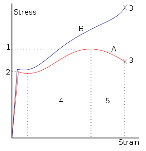 Stress–strain curve for low-carbon steel. Hooke's law is only valid for the portion of the curve between the origin and the yield point(2).
1. Ultimate strength
2. Yield strength – corresponds to yield point
3. Rupture
4. Strain hardening region
5. Necking region
A: (F/A0)
B: True stress (F/A)The most commonly encountered form of Hooke's law is probably the spring equation, which relates the force exerted by a spring to the distance it is stretched by a spring constant, k, measured in force per length.
The negative sign indicates that the force exerted by the spring is in direct opposition to the direction of displacement. It is called a "restoring force", as it tends to restore the system to equilibrium. The potential energy stored in a spring is given by
which comes from adding up the energy it takes to incrementally compress the spring. That is, the integral of force over displacement. (Note that potential energy of a spring is always non-negative.)
This potential can be visualized as a parabola on the U-x plane. As the spring is stretched in the positive x-direction, the potential energy increases (the same thing happens as the spring is compressed). The corresponding point on the potential energy curve is higher than that corresponding to the equilibrium position (x = 0). The tendency for the spring is to therefore decrease its potential energy by returning to its equilibrium (unstretched) position, just as a ball rolls downhill to decrease its gravitational potential energy.
If a mass m is attached to the end of such a spring, the system becomes a harmonic oscillator. It will oscillate with a natural frequency given either as an angular frequency
or as a natural frequency
This idealized description of spring mechanics works as long as the mass of the spring is very small compared to the mass m, there is no significant friction on the system, and the spring is not overextended beyond its natural range (which can deform it permanently).
Multiple springs
When two springs are attached to a mass and compressed, the following table compares values of the springs.
Comparison In Parallel In Series 

Equivalent
spring constant

Compressed
distance

Energy
stored

Derivation
-
Equivalent Spring Constant (Series) Defining the displacement from the equilibrium position of the block to be x2, we'll be looking for an equation for the force on the block that looks like: To begin, we'll also define the displacement from the equilibrium position of the point between the two springs to be x1.
The force on the block is
Meanwhile, the force on the point between the two springs is
Now, when the block is pushed so the springs are compressed and the system is allowed to come to equilibrium, the force between the springs must sum to zero, so with Fs = 0 we can solve for
 :
:so
Now we just plug this back into (1):
Finally, the force on the block has been found:
So we can define everything in the parenthesis to be
Which can also be written:
-
-
Equivalent Spring Constant (Parallel) Both springs are touching the block in this case, and whatever distance spring 1 is compressed has to be the same amount spring 2 is compressed. The force on the block is then:
So the force on the block is
Which is why we can define the equivalent spring constant as
-
-
Compressed Distance In the case where two springs are in series, the magnitude of the force of the springs on each other are equal: For spring 1, x1 is the distance from equilibrium length, and for spring 2, x2 – x1 is the distance from its equilibrium length. So we can define
Plug these definitions into the force equation, and we'll get a relationship between the compressed distances for the in series case:
-
-
Energy Stored For the series case, the ratio of energy stored in springs is: but there is a relationship between a1 and a2 derived earlier, so we can plug that in:
For the parallel case,
because the compressed distance of the springs is the same, this simplifies to
-
Tensor expression of Hooke's Law
- Note: the Einstein summation convention of summing on repeated indices is used below.
When working with a three-dimensional stress state, a 4th order tensor (
( ) containing 81 elastic coefficients must be defined to link the stress tensor
  (σij) and the strain tensor
  (
( ).
).Expressed in terms of components with respect to an orthonormal basis, the generalized form of Hooke's law is written as (using the summation convention)
The tensor
is called the stiffness tensor or the elasticity tensor. Due to the symmetry of the stress tensor, strain tensor, and stiffness tensor, only 21 elastic coefficients are independent. As stress is measured in units of pressure and strain is dimensionless, the entries of are also in units of pressure.The expression for generalized Hooke's law can be inverted to get a relation for the strain in terms of stress:
The tensor
 is called the compliance tensor.
Generalization for the case of large deformations is provided by models of neo-Hookean solids and Mooney-Rivlin solids.
Isotropic materials
(see viscosity for an analogous development for viscous fluids.)
Isotropic materials are characterized by properties which are independent of direction in space. Physical equations involving isotropic materials must therefore be independent of the coordinate system chosen to represent them. The strain tensor is a symmetric tensor. Since the trace of any tensor is independent of any coordinate system, the most complete coordinate-free decomposition of a symmetric tensor is to represent it as the sum of a constant tensor and a traceless symmetric tensor.[4]:Ch. 10 Thus:
where δij is the Kronecker delta. In direct tensor notation
where
 is the second-order identity tensor. The first term on the right is the constant tensor, also known as the volumetric strain tensor, and the second term is the traceless symmetric tensor, also known as the deviatoric strain tensor or shear tensor.
The most general form of Hooke's law for isotropic materials may now be written as a linear combination of these two tensors:
where K is the bulk modulus and G is the shear modulus.
Using the relationships between the elastic moduli, these equations may also be expressed in various other ways. A common form of Hooke's law for isotropic materials, expressed in direct tensor notation, is [5]
where λ: = K − 2 / 3G and μ: = G are the Lamé constants,
is the second-order identity tensor, and  is the symmetric part of the fourth-order identity tensor. In terms of components with respect to a Cartesian basis,
The inverse relationship is[6]
Therefore the compliance tensor in the relation
 is
isIn terms of Young's modulus and Poisson's ratio, Hooke's law for isotropic materials can then be expressed as
This is the form in which the strain is expressed in terms of the stress tensor in engineering. The expression in expanded form is
where E is the modulus of elasticity and ν is Poisson's ratio. (See 3-D elasticity).
-
Derivation of Hooke's law in 3D The 3-D form of Hooke's law can be derived using Poisson's ratio and the 1-D form of Hooke's law as follows. Consider the strain and stress relation as a superposition of two effects: stretching in direction of the load (1) and shrinking (caused by the load) in perpendicular directions (2 and 3),
 ,
, ,
, ,
,
where ν is the Poisson's ratio and E the Young Modulus. We get similar equations to the loads in directions 2 and 3,
 ,
, ,
, ,
,
and
 ,
, ,
, .
.
Summing the three cases together (εi = εi' + εi'' + εi''') we get
or by adding and subtracting one νσ
and further we get by solving σ1
 .
.
Calculating the sum
and substituting it to the equation solved for σ1 gives
 ,
,- σ1 = 2με1 + λ(ε1 + ε2 + ε3),
where μ and λ are the Lamé parameters. Similar treatment of directions 2 and 3 gives the Hooke's law in three dimensions.
In matrix form, Hooke's law for isotropic materials can be written as
where γij: = 2εij is the engineering shear strain. The inverse relation may be written as
which expression can be simplified thanks to the Lamé constants :
Plane stress Hooke's law
Under plane stress conditions σ33 = σ31 = σ13 = σ32 = σ23 = 0. In that case Hooke's law takes the form
The inverse relation is usually written in the reduced form
Anisotropic materials
The symmetry of the Cauchy stress tensor (
 ) and the generalized Hooke's laws (
 ) implies that
  . Similarly, the symmetry of the infinitesimal strain tensor implies that
  . These symmetries are called the minor symmetries of the stiffness tensor ().
If in addition, since the displacement gradient and the Cauchy stress are work conjugate, the stress-strain relation can be derived from a strain energy density functional (U), then
The arbitrariness of the order of differentiation implies that
 . These are called the major symmetries of the stiffness tensor. The major and minor symmetries indicate that the stiffness tensor has only 21 independent components.
Matrix representation (stiffness tensor)
It is often useful to express the anisotropic form of Hooke's law in matrix notation, also called Voigt notation. To do this we take advantage of the symmetry of the stress and strain tensors and express them as six-dimensional vectors in an orthonormal coordinate system (
 ) as
) asThen the stiffness tensor (
) can be expressed asand Hooke's law is written as
Similarly the compliance tensor (
) can be written asChange of coordinate system
If a linear elastic material is rotated from a reference configuration to another, then the material is symmetric with respect to the rotation if the components of the stiffness tensor in the rotated configuration are related to the components in the reference configuration by the relation[7]
where lab are the components of an orthogonal rotation matrix [L]. The same relation also holds for inversions.
In matrix notation, if the transformed basis (rotated or inverted) is related to the reference basis by
then
In addition, if the material is symmetric with respect to the transformation [L] then
Orthotropic materials
Main article: Orthotropic materialOrthotropic materials have three orthogonal planes of symmetry. If the basis vectors (
) are normals to the planes of symmetry then the coordinate transformation relations imply thatThe inverse of this relation is commonly written as[8]
where
 is the Young's modulus along axis i
 is the shear modulus in direction j on the plane whose normal is in direction i
 is the Poisson's ratio that corresponds to a contraction in direction j when an extension is applied in direction i.
Under plane stress conditions, σzz = σzx = σyz = 0, Hooke's law for an orthotropic material takes the form
The inverse relation is
The transposed form of the above stiffness matrix is also often used.
Transversely isotropic materials
A transversely isotropic material is symmetric with respect to a rotation about an axis of symmetry. For such a material, if
 is the axis of symmetry, Hooke's law can be expressed as
More frequently, the
 axis is taken to be the axis of symmetry and the inverse Hooke's law is written as [9]
Thermodynamic basis of Hooke's law
Linear deformations of elastic materials can be approximated as adiabatic. Under these conditions and for quasistatic processes the first law of thermodynamics for a deformed body can be expressed as
where δU is the increase in internal energy and δW is the work done by external forces. The work can be split into two terms
where δWs is the work done by surface forces while δWb is the work done by body forces. If
 is a variation of the displacement field
  in the body, then the two external work terms can be expressed as
where
 is the surface traction vector,
  is the body force vector,
  represents the body and
  represents its surface. Using the relation between the Cauchy stress and the surface traction,
  (where
  is the unit outward normal to ), we have
Converting the surface integral into a volume integral via the divergence theorem gives
Using the symmetry of the Cauchy stress and the identity
we have
From the definition of strain and from the equations of equilibrium we have
Hence we can write
and therefore the variation in the internal energy density is given by
An elastic material is defined as one in which the total internal energy is equal to the potential energy of the internal forces (also called the elastic strain energy). Therefore the internal energy density is a function of the strains,
 and the variation of the internal energy can be expressed as
Since the variation of strain is arbitrary, the stress-strain relation of an elastic material is given by
For a linear elastic material, the quantity
 is a linear function of , and can therefore be expressed as
where
is a fourth-order tensor of material constants, also called the stiffness tensor. We can see why must be a fourth-order tensor by noting that, for a linear elastic material,In index notation
Clearly, the right hand side constant requires four indices and is a fourth-order quantity. We can also see that this quantity must be a tensor because it is a linear transformation that takes the strain tensor to the stress tensor. We can also show that the constant obeys the tensor transformation rules for fourth order tensors.
See also
Continuum mechanics  LawsSolids
Stress · Deformation
Compatibility
Finite strain · Infinitesimal strain
Elasticity (linear) · Plasticity
Bending · Hooke's law
Failure theory
Fracture mechanics
Frictionless/Frictional Contact mechanicsScientists- Elasticity (physics)
- Elastic limit
- Elastic modulus
- Elastic potential energy
- Infinitesimal strain theory
- List of scientific laws named after people
- Linear elasticity
- Quadratic form
- Spring system
- Poisson's ratio
- Simple harmonic motion of a mass on a spring
- Sine wave
- Solid mechanics
- Stress (mechanics)
Notes
- ^ Walter Lewin (1 October 1999) (in English) (ogg). Hook's Law, Simple Harmonic Oscillator. MIT Course 8.01: Classical Mechanics, Lecture 10. (videotape). Cambridge, MA USA: MIT OCW. Event occurs at 1:21–10:10. http://ocw.mit.edu/courses/physics/8-01-physics-i-classical-mechanics-fall-1999/video-lectures/lecture-10/. Retrieved 23 December 2010. "...arguably the most important equation in all of Physics."
- ^ Walter Lewin (1 October 1999) (in English) (ogg). Hook's Law, Simple Harmonic Oscillator. MIT Course 8.01: Classical Mechanics, Lecture 10. (videotape). Cambridge, MA USA: MIT OCW. Event occurs at 10:10–16:33. http://ocw.mit.edu/courses/physics/8-01-physics-i-classical-mechanics-fall-1999/video-lectures/lecture-10/. Retrieved 23 December 2010.
- ^ The anagram was "ceiiinosssttuv", [1]; cf. the anagram for the Catenary, which appeared in the preceding paragraph.
- ^ Symon, Keith (1971). Mechanics. Addison-Wesley, Reading, MA. ISBN 0-201-07392-7.
- ^ Simo, J. C. and Hughes, T. J. R., 1998, Computational Inelasticity, Springer.
- ^ Milton, G. W., 2002, Theory of Composites, Cambridge University Press.
- ^ Slaughter, W. S., 2002, The Linearized Theory of Elasticity, Birkhauser
- ^ Boresi, A. P, Schmidt, R. J. and Sidebottom, O. M., 1993, Advanced Mechanics of Materials, Wiley.
- ^ Tan, S. C., 1994, Stress Concentrations in Laminated Composites, Technomic Publishing Company, Lancaster, PA.
References
- A.C. Ugural, S.K. Fenster, Advanced Strength and Applied Elasticity, 4th ed
External links
Elastic moduli for homogeneous isotropic materials Bulk modulus (K) · Young's modulus (E) · Lamé's first parameter (λ) · Shear modulus (G) · Poisson's ratio (ν) · P-wave modulus (M)Conversion formulas Homogeneous isotropic linear elastic materials have their elastic properties uniquely determined by any two moduli among these, thus given any two, any other of the elastic moduli can be calculated according to these formulas. 


 Categories:
- Springs (mechanical)
- Elasticity (physics)
- Solid mechanics


![\boldsymbol{\varepsilon} = \tfrac{1}{E}~\boldsymbol{\sigma} - \tfrac{\nu}{E}\left[\mathrm{tr}(\boldsymbol{\sigma})~\mathbf{I} - \boldsymbol{\sigma}\right]](c/bac6b0cd7365a2bd4d1237dd489988f4.png)
![\begin{align}
\varepsilon_{11} & = \tfrac{1}{E}\left[ \sigma_{11} - \nu(\sigma_{22}+\sigma_{33}) \right] \\
\varepsilon_{22} & = \tfrac{1}{E}\left[\sigma_{22} - \nu(\sigma_{11}+\sigma_{33}) \right] \\
\varepsilon_{33} & = \tfrac{1}{E}\left[\sigma_{33} - \nu(\sigma_{11}+\sigma_{22}) \right] \\
\varepsilon_{12} & = \tfrac{1}{2G}~\sigma_{12} ~;~~
\varepsilon_{13} = \tfrac{1}{2G}~\sigma_{13} ~;~~
\varepsilon_{23} = \tfrac{1}{2G}~\sigma_{23}
\end{align}](3/5a3d175ea26c4458e3094e580dade13a.png)


![[\boldsymbol{\sigma}] = \begin{bmatrix}\sigma_{11}\\ \sigma_{22} \\ \sigma_{33} \\ \sigma_{23} \\ \sigma_{31} \\ \sigma_{12} \end{bmatrix} \equiv
\begin{bmatrix} \sigma_1 \\ \sigma_2 \\ \sigma_3 \\ \sigma_4 \\ \sigma_5 \\ \sigma_6 \end{bmatrix} ~;~~
[\boldsymbol{\epsilon}] = \begin{bmatrix}\epsilon_{11}\\ \epsilon_{22} \\ \epsilon_{33} \\ 2\epsilon_{23} \\ 2\epsilon_{31} \\ 2\epsilon_{12} \end{bmatrix} \equiv
\begin{bmatrix} \epsilon_1 \\ \epsilon_2 \\ \epsilon_3 \\ \epsilon_4 \\ \epsilon_5 \\ \epsilon_6 \end{bmatrix}](e/04e576989af699b7569633e0730db54e.png)
![[\mathsf{C}] = \begin{bmatrix} c_{1111} & c_{1122} & c_{1133} & c_{1123} & c_{1131} & c_{1112} \\
c_{2211} & c_{2222} & c_{2233} & c_{2223} & c_{2231} & c_{2212} \\
c_{3311} & c_{3322} & c_{3333} & c_{3323} & c_{3331} & c_{3312} \\
c_{2311} & c_{2322} & c_{2333} & c_{2323} & c_{2331} & c_{2312} \\
c_{3111} & c_{3122} & c_{3133} & c_{3123} & c_{3131} & c_{3112} \\
c_{1211} & c_{1222} & c_{1233} & c_{1223} & c_{1231} & c_{1212}
\end{bmatrix} \equiv \begin{bmatrix}
C_{11} & C_{12} & C_{13} & C_{14} & C_{15} & C_{16} \\
C_{12} & C_{22} & C_{23} & C_{24} & C_{25} & C_{26} \\
C_{13} & C_{23} & C_{33} & C_{34} & C_{35} & C_{36} \\
C_{14} & C_{24} & C_{34} & C_{44} & C_{45} & C_{46} \\
C_{15} & C_{25} & C_{35} & C_{45} & C_{55} & C_{56} \\
C_{16} & C_{26} & C_{36} & C_{46} & C_{56} & C_{66} \end{bmatrix}](4/b04f02b5b99678d04f6717616c740d3c.png)
![[\boldsymbol{\sigma}] = [\mathsf{C}][\boldsymbol{\epsilon}] \qquad \text{or} \qquad \sigma_i = C_{ij} \epsilon_j ~.](4/2145b36b5d0f26004444f2c708f3629a.png)
![[\mathsf{S}] = \begin{bmatrix}
s_{1111} & s_{1122} & s_{1133} & 2s_{1123} & 2s_{1131} & 2s_{1112} \\
s_{2211} & s_{2222} & s_{2233} & 2s_{2223} & 2s_{2231} & 2s_{2212} \\
s_{3311} & s_{3322} & s_{3333} & 2s_{3323} & 2s_{3331} & 2s_{3312} \\
2s_{2311} & 2s_{2322} & 2s_{2333} & 4s_{2323} & 4s_{2331} & 4s_{2312} \\
2s_{3111} & 2s_{3122} & 2s_{3133} & 4s_{3123} & 4s_{3131} & 4s_{3112} \\
2s_{1211} & 2s_{1222} & 2s_{1233} & 4s_{1223} & 4s_{1231} & 4s_{1212}
\end{bmatrix} \equiv \begin{bmatrix}
S_{11} & S_{12} & S_{13} & S_{14} & S_{15} & S_{16} \\
S_{12} & S_{22} & S_{23} & S_{24} & S_{25} & S_{26} \\
S_{13} & S_{23} & S_{33} & S_{34} & S_{35} & S_{36} \\
S_{14} & S_{24} & S_{34} & S_{44} & S_{45} & S_{46} \\
S_{15} & S_{25} & S_{35} & S_{45} & S_{55} & S_{56} \\
S_{16} & S_{26} & S_{36} & S_{46} & S_{56} & S_{66} \end{bmatrix}](8/868fe27ec384ff66d00a92a9e54e2909.png)

![[\mathbf{e}_i'] = [L][\mathbf{e}_i]](3/dd3cc47ec20e90dbb73168820fdbf6f0.png)


![\delta U = \int_{\Omega} [\boldsymbol{\nabla}\cdot(\boldsymbol{\sigma}\cdot\delta\mathbf{u}) + \mathbf{b}\cdot\delta\mathbf{u}]~ {\rm dV} ~.](f/c9f9f13d353b29bc52ebd0ee70a6c09a.png)
![\boldsymbol{\nabla}\cdot(\boldsymbol{A}\cdot\mathbf{b}) = (\boldsymbol{\nabla}\cdot\boldsymbol{A})\cdot\mathbf{b}+
\tfrac{1}{2}[\boldsymbol{A}^T:\boldsymbol{\nabla}\mathbf{b}+
\boldsymbol{A}:(\boldsymbol{\nabla}\mathbf{b})^T]](9/de94ab3092064dd2eaca26635c286f37.png)
![\delta U = \int_{\Omega} [\boldsymbol{\sigma}:
\tfrac{1}{2}\{\boldsymbol{\nabla}\delta\mathbf{u}+(\boldsymbol{\nabla}\delta\mathbf{u})^T\} + \{\boldsymbol{\nabla}\cdot\boldsymbol{\sigma}+\mathbf{b}\}\cdot\delta\mathbf{u}]~{\rm dV} ~.](7/28727c2be4bd632f93992dad27004c78.png)
![\delta\boldsymbol{\epsilon} = \tfrac{1}{2}[\boldsymbol{\nabla}\delta\mathbf{u}+(\boldsymbol{\nabla}\delta\mathbf{u})^T] ~;~~
\boldsymbol{\nabla}\cdot\boldsymbol{\sigma}+\mathbf{b}=\mathbf{0} ~.](b/61bbdb60116732bdd4909d29f1080180.png)


![\cfrac{\partial}{\partial\boldsymbol{\epsilon}}[\boldsymbol{\sigma}(\boldsymbol{\epsilon})] = \text{constant} = \mathsf{c} \,.](a/8bae5968bbfb48b4e8bebbff6aad13c1.png)


Wikimedia Foundation. 2010.