Astronomical seeing

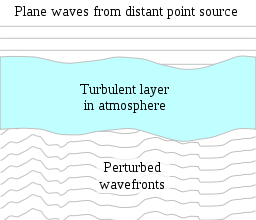Schematic diagram illustrating how optical wavefronts from a distant star may be perturbed by a layer of turbulent mixing in the atmosphere. The vertical scale of the wavefronts plotted is highly exaggerated.

Astronomical seeing refers to the blurring and twinkling of astronomical objects such as stars caused by turbulent mixing in the Earth's atmosphere varying the optical refractive index. The astronomical seeing conditions on a given night at a given location describe how much the Earth's atmosphere perturbs the images of stars as seen through a telescope.

The most common seeing measurement is the diameter (technically full width at half maximum or FWHM) of the seeing disc (the point spread function for imaging through the atmosphere). The point spread function diameter (seeing disc diameter or "seeing") is a reference to the best possible angular resolution which can be achieved by an optical telescope in a long photographic exposure, and corresponds to the diameter of the fuzzy blob seen when observing a point-like star through the atmosphere. The size of the seeing disc is determined by the astronomical seeing conditions at the time of the observation. The best conditions give a seeing disk diameter of ~0.4 arcseconds and are found at high-altitude observatories on small islands such as Mauna Kea or La Palma.

Seeing is one of the biggest problems for Earth-based astronomy: while the big telescopes have theoretically milli-arcsecond resolution, the real image will never be better than the average seeing disc during the observation. This can easily mean a factor of 100 between the potential and practical resolution. Starting in the 1990s, new adaptive optics have been introduced that can help correct for these effects, dramatically improving the resolution of ground based telescopes.

The image fluctuations seen when looking at the bottom of a lake on a windy day are caused by refractive index fluctuations, but in the case of a lake they do not result from turbulent mixing.

The effects of astronomical seeing

• 

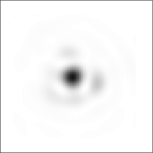
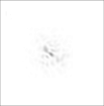
  Typical short-exposure negative image of a binary star (Zeta Boötis in this case) as seen through atmospheric seeing. Each star should appear as a single Airy pattern, but the atmosphere causes the images of the two stars to break up into two patterns of speckles (one pattern above left, the other below right). The speckles are a little difficult to make out in this image due to the coarse pixel size on the camera used (see the simulated images below for a clearer example). The speckles move around rapidly, so that each star appears as a single fuzzy blob in long exposure images (called a seeing disc). The telescope used had a diameter of about 7r₀ (see definition of r₀ below, and example simulated image through a 7r₀ telescope).

Astronomical seeing has several effects:

1. It causes the images of point sources (such as stars), which in the absence of atmospheric turbulence would be steady Airy patterns produced by diffraction, to break up into speckle patterns, which change very rapidly with time (the resulting speckled images can be processed using speckle imaging)
2. Long exposure images of these changing speckle patterns result in a blurred image of the point source, called a seeing disc
3. The brightness of stars appears to fluctuate in a process known as scintillation or twinkling
4. Atmospheric seeing causes the fringes in an astronomical interferometer to move rapidly
5. The distribution of atmospheric seeing through the atmosphere (the C_N² profile described below) causes the image quality in adaptive optics systems to degrade the further you look from the location of reference star

The effects of atmospheric seeing were indirectly responsible for the belief that there were canals on Mars.^{[citation needed]} In viewing a bright object such as Mars, occasionally a still patch of air will come in front of the planet, resulting in a brief moment of clarity. Before the use of charge-coupled devices, there was no way of recording the image of the planet in the brief moment other than having the observer remember the image and draw it later. This had the effect of having the image of the planet be dependent on the observer's memory and preconceptions which led the belief that Mars had linear features.

The effects of atmospheric seeing are qualitatively similar throughout the visible and near infra-red wavebands. At large telescopes the long exposure image resolution is generally slightly higher at longer wavelengths, and the timescale (t₀ - see below) for the changes in the dancing speckle patterns is substantially lower.

Measures of astronomical seeing

There are three common descriptions of the astronomical seeing conditions at an observatory:

1. The FWHM of the seeing disc
2. r₀ (the size of a typical "lump" of uniform air within the turbulent atmosphere^[1]) and t₀ (the time-scale over which the changes in the turbulence become significant)
3. The C_N² profile

These are described in the sub-sections below:

The full width at half maximum (FWHM) of the seeing disc

Without an atmosphere, a small star would have an apparent size, an "Airy disk", in a telescope image determined by diffraction and would be inversely proportional to the diameter of the telescope. However when light enters the Earth's atmosphere, the different temperature layers and different wind speeds distort the light waves leading to distortions in the image of a star. The effects of the atmosphere can be modeled as rotating cells of air moving turbulently. At most observatories the turbulence is only significant on scales larger than r₀ (see below—the seeing parameter r₀ is 10–20 cm at visible wavelengths under the best conditions) and this limits the resolution of telescopes to be about the same as given by a space-based 10–20 cm telescope.

The distortion changes at a high rate, typically more frequently than 100 times a second. In a typical astronomical image of a star with an exposure time of seconds or even minutes, the different distortions average out as a filled disc called the point spread function or "seeing disc". The diameter of the seeing disk, most often defined as the full width at half maximum (FWHM), is a measure of the astronomical seeing conditions.

It follows from this definition that seeing is always a variable quantity, different from place to place, from night to night and even variable on a scale of minutes. Astronomers often talk about "good" nights with a low average seeing disc diameter, and "bad" nights where the seeing diameter was so high that all observations were worthless.

• 

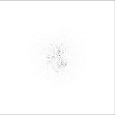
  Slow motion movie of what you see through a telescope when you look at a star at high magnification (negative images). The telescope used had a diameter of about 7r₀ (see definition of r₀ below, and example simulated image through a 7r₀ telescope). Notice how the star breaks up into multiple blobs (speckles) -- entirely an atmospheric effect. Some telescope vibration is also noticeable.

The FWHM of the seeing disc (or just Seeing) is usually measured in arcseconds, abbreviated with the symbol ("). A 1.0" seeing is a good one for average astronomical sites. The seeing of an urban environment is usually much worse. Good seeing nights tend to be clear, cold nights without wind gusts. Warm air rises (convection) degrading the seeing as does wind and clouds. At the best high-altitude mountaintop observatories the wind brings in stable air which has not previously been in contact with the ground, sometimes providing seeing as good as 0.4".

r₀ and t₀

The astronomical seeing conditions at an observatory can be well described by the parameters r₀ and t₀. For telescopes with diameters smaller than r₀, the resolution of long-exposure images is determined primarily by diffraction and the size of the Airy pattern and thus is inversely proportional to the telescope diameter. For telescopes with diameters larger than r₀, the image resolution determined primarily by the atmosphere and is independent of telescope diameter, remaining constant at the value given by a telescope of diameter equal to r₀. r₀ also corresponds to the length-scale over which the turbulence becomes significant (10–20 cm at visible wavelengths at good observatories), and t₀ corresponds to the time-scale over which the changes in the turbulence become significant. r₀ determines the spacing of the actuators needed in an active optics system, and t₀ determines the correction speed required to compensate for the effects of the atmosphere.

r₀ and t₀ vary with the wavelength used for the astronomical imaging, allowing slightly higher resolution imaging at longer wavelengths using large telescopes.

r₀ is often known as the Fried parameter (pronounced freed), named after David L. Fried.

Mathematical description of r₀ and t₀

Simulated negative image showing what a single (point-like) star would look like through a ground-based telescope with a diameter of 2r₀. The blurred look of the image is because of diffraction, which causes the appearance of the star to be an Airy pattern with a central disk surrounded by hints of faint rings. The atmosphere would make the image move around very rapidly, so that in a long-exposure photograph it would appear more blurred.

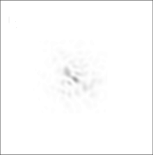Simulated negative image showing what a single (point-like) star would look like through a ground-based telescope with a diameter of 7r₀, on the same angular scale as the 2r₀ image above. The atmosphere makes the image break up into several blobs (speckles). The speckles move around very rapidly, so that in a long-exposure photograph the star would appear as a single blurred blob.

Simulated negative image showing what a single (point-like) star would look like through a ground-based telescope with a diameter of 20r₀. The atmosphere makes the image break up into several blobs (speckles). The speckles move around very rapidly, so that in a long-exposure photograph the star would appear as a single blurred blob.

Mathematical models can give an accurate model of the effects of astronomical seeing on images taken through ground-based telescopes. Three simulated short-exposure images are shown at the right through three different telescope diameters (as negative images to highlight the fainter features more clearly—a common astronomical convention). The telescope diameters are quoted in terms of the Fried parameter r₀ (defined below). r₀ is a commonly used measurement of the astronomical seeing at observatories. At visible wavelengths, r₀ varies from 20 cm at the best locations to 5 cm at typical sea-level sites.

In reality the pattern of blobs (speckles) in the images changes very rapidly, so that long exposure photographs would just show a single large blurred blob in the centre for each telescope diameter. The diameter (FWHM) of the large blurred blob in long exposure images is called the seeing disc diameter, and is independent of the telescope diameter used (as long as adaptive optics correction is not applied).

It is first useful to give a brief overview of the basic theory of optical propagation through the atmosphere. In the standard classical theory, light is treated as an oscillation in a field ψ. For monochromatic plane waves arriving from a distant point source with wave-vector $\mathbf{k}$: $\psi_{0} \left(\mathbf{r},t\right) = A_{u}e^{i\left (\phi_{u} + 2\pi\nu t + \mathbf{k}\cdot\mathbf{r} \right )}$ where ψ₀ is the complex field at position $\mathbf{r}$ and time t, with real and imaginary parts corresponding to the electric and magnetic field components, ϕ_u represents a phase offset, ν is the frequency of the light determined by $\nu=c\left | \mathbf{k} \right | / \left ( 2 \pi \right )$, and A_u is the amplitude of the light.

The photon flux in this case is proportional to the square of the amplitude A_u, and the optical phase corresponds to the complex argument of ψ₀. As wavefronts pass through the Earth's atmosphere they may be perturbed by refractive index variations in the atmosphere. The diagram at the top-right of this page shows schematically a turbulent layer in the Earth's atmosphere perturbing planar wavefronts before they enter a telescope. The perturbed wavefront ψ_p may be related at any given instant to the original planar wavefront $\psi_{0} \left(\mathbf{r}\right)$ in the following way: $\psi_{p} \left(\mathbf{r}\right) = \left ( \chi_{a} \left(\mathbf{r}\right) e^{i\phi_{a} \left(\mathbf{r}\right)}\right ) \psi_{0} \left(\mathbf{r}\right)$

where $\chi_{a} \left(\mathbf{r}\right)$ represents the fractional change in wavefront amplitude and $\phi_{a} \left(\mathbf{r}\right)$ is the change in wavefront phase introduced by the atmosphere. It is important to emphasise that $\chi_{a} \left(\mathbf{r}\right)$ and $\phi_{a} \left(\mathbf{r}\right)$ describe the effect of the Earth's atmosphere, and the timescales for any changes in these functions will be set by the speed of refractive index fluctuations in the atmosphere.

The Kolmogorov model of turbulence

A description of the nature of the wavefront perturbations introduced by the atmosphere is provided by the Kolmogorov model developed by Tatarski,^[2] based partly on the studies of turbulence by the Russian mathematician Andreï Kolmogorov.^[3] This model is supported by a variety of experimental measurements^[4] and is widely used in simulations of astronomical imaging. The model assumes that the wavefront perturbations are brought about by variations in the refractive index of the atmosphere. These refractive index variations lead directly to phase fluctuations described by $\phi_{a} \left(\mathbf{r}\right)$, but any amplitude fluctuations are only brought about as a second-order effect while the perturbed wavefronts propagate from the perturbing atmospheric layer to the telescope. For all reasonable models of the Earth's atmosphere at optical and infra-red wavelengths the instantaneous imaging performance is dominated by the phase fluctuations $\phi_{a} \left(\mathbf{r}\right)$. The amplitude fluctuations described by $\chi_{a} \left(\mathbf{r}\right)$ have negligible effect on the structure of the images seen in the focus of a large telescope.

For simplicity, the phase fluctuations in Tatarski's model are often assumed to have a Gaussian random distribution with the following second order structure function: $D_{\phi_{a}}\left(\mathbf{\rho} \right) = \left \langle \left | \phi_{a} \left ( \mathbf{r} \right ) - \phi_{a} \left ( \mathbf{r} + \mathbf{\rho} \right ) \right | ^{2} \right \rangle _{\mathbf{r}}$

where $D_{\phi_{a}} \left ({\mathbf{\rho}} \right )$ is the atmospherically induced variance between the phase at two parts of the wavefront separated by a distance $\mathbf{\rho}$ in the aperture plane, and < ... > represents the ensemble average.

For the Gaussian random approximation, the structure function of Tatarski (1961) can be described in terms of a single parameter r₀:

$D_{\phi_{a}} \left ({\mathbf{\rho}} \right ) = 6.88 \left ( \frac{\left | \mathbf{\rho} \right |}{r_{0}} \right ) ^{5/3}$

r₀ indicates the strength of the phase fluctuations as it corresponds to the diameter of a circular telescope aperture at which atmospheric phase perturbations begin to seriously limit the image resolution. Typical r₀ values for I band (900 nm wavelength) observations at good sites are 20---40 cm. It should be noted^[5] that r₀ also corresponds to the aperture diameter for which the variance σ² of the wavefront phase averaged over the aperture comes approximately to unity: $\sigma ^{2}=1.0299 \left ( \frac{d}{r_{0}} \right )^{5/3}$

This equation represents a commonly used definition for r₀, a parameter frequently used to describe the atmospheric conditions at astronomical observatories.

r₀ can be determined from a measured C_N² profile (described below) as follows:

$r_{0}=\left ( 16.7\lambda^{-2}( \cos \gamma )^{-1}\int_{0}^{\infty}dh C_{N}^{2}(h) \right )^{-3/5}$

where the turbulence strength $C_{N}^{2}(h)$ varies as a function of height h above the telescope, and γ is the angular distance of the astronomical source from the zenith (from directly overhead).

If turbulent evolution is assumed to occur on slow timescales, then the timescale t₀ is simply proportional to r₀ divided by the mean wind speed.

The refractive index fluctuations caused by Gaussian random turbulence can be simulated using the following algorithm^[6]:

$\phi_a (\mathbf{r})=\mbox{Re}[\mbox{FT}[R(\mathbf{k})K(\mathbf{k})]]$

where $\phi_a(\mathbf{r})$ is the optical phase error introduced by atmospheric turbulence, R (k) is a 2 dimensional square array of independent random complex numbers which have a Gaussian distribution about zero and white noise spectrum, K (k) is the (real) Fourier amplitude expected from the Kolmogorov (or Von Karman) spectrum, Re[] represents taking the real part, and FT[] represents a discrete Fourier transform of the resulting 2 dimensional square array (typically an FFT).

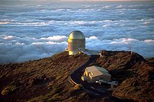Astronomical observatories are generally situated on mountaintops, as the air at ground level is usually more convective. A light wind bringing stable air from high above the clouds and ocean generally provides the best seeing conditions (telescope shown: NOT).

Turbulent intermittency

The assumption that the phase fluctuations in Tatarski's model have a Gaussian random distribution is usually unrealistic. In reality turbulence exhibits intermittency^[7]

These fluctuations in the turbulence strength can be straightforwardly simulated as follows:^[8]:

$\phi_a (\mathbf{r})=\mbox{Re}[\mbox{FT}[(R(\mathbf{k})\otimes I(\mathbf{k}))K(\mathbf{k})]]$

where I (k) is a 2 dimensional array which represents the spectrum of intermittency, with the same dimensions as R (k), and where $\otimes$ represents convolution. The intermittency is described in terms of fluctuations in the turbulence strength $C_n^2$. It can be seen the equation for the Gaussian random case above is just the special case from this equation with:

I(k) = δ( | k | )

where δ() is the Dirac delta function.

The $C_n^2$ profile

A more thorough description of the astronomical seeing at an observatory is given by producing a profile of the turbulence strength as a function of altitude, called a $C_n^2$ profile. $C_n^2$ profiles are generally performed when deciding on the type of adaptive optics system which will be needed at a particular telescope, or in deciding whether or not a particular location would be a good site for setting up a new astronomical observatory. Typically, several methods are used simultaneously for measuring the $C_n^2$ profile and then compared. Some of the most common methods include:

1. SCIDAR (imaging the shadow patterns in the scintillation of starlight)
2. LOLAS (a small aperture variant of SCIDAR designed for low-altitude profiling)
3. SLODAR
4. MASS
5. RADAR mapping of turbulence
6. Balloon-borne thermometers to measure how quickly the air temperature is fluctuating with time due to turbulence

There are also mathematical functions describing the $C_n^2$ profile. Some are empirical fits from measured data and others attempt to incorporate elements of theory. One common model for continental land masses is known as Hufnagel-Valley after two workers in this subject.

Overcoming atmospheric seeing

An animated image of the Moon's surface showing the effects of Earth's atmosphere on the view

The first answer to this problem was speckle imaging, which allowed bright objects to be observed with very high resolution. Later came NASA's Hubble Space Telescope, working outside the atmosphere and thus not having any seeing problems and allowing observations of faint targets for the first time (although with poorer resolution than speckle observations of bright sources from ground-based telescopes because of Hubble's smaller telescope diameter). The highest resolution visible and infrared images currently come from imaging optical interferometers such as the Navy Prototype Optical Interferometer or Cambridge Optical Aperture Synthesis Telescope.

Starting in the 1990s, many telescopes have begun to develop adaptive optics systems that partially solve the seeing problem, but none of the systems so far built or designed completely removes the atmosphere effect, and observations are usually limited to a small region of the sky surrounding relatively bright stars.

Another cheaper technique, lucky imaging, has had very good results. This idea dates back to pre-war naked-eye observations of moments of good seeing, which were followed by observations of the planets on cine film after World War II. The technique relies on the fact that every so often the effects of the atmosphere will be negligible, and hence by recording large numbers of images in real-time, a 'lucky' excellent image can be picked out. This technique can outperform adaptive optics in many cases and is even accessible to amateurs. It does, however, require very much longer observation times than adaptive optics for imaging faint targets, and is limited in its maximum resolution.

See also

• The Royal Astronomical Society of Canada Calgary Centre - Atmospheric "Seeing". Includes animated illustrations of effects of seeing.
• Atmosphere and Telescope Simulator - Atmospheric turbulence simulator.
• Clear Sky Chart - includes a weather forecast of astronomical seeing.
• Mirage
• Transient lunar phenomenon

References

Much of the above text is taken (with permission) from Lucky Exposures: Diffraction limited astronomical imaging through the atmosphere, by Robert Nigel Tubbs

1. ^ To Measure the Sky: An Introduction to Observational Astronomy by Frederick R. Chromey, Cambridge University Press, 2010, page 140.
2. ^ *TATARSKI, V. I. (1961). Wave Propagation in a Turbulent Medium. McGraw-Hill Books. 
3. ^
   • KOLMOGOROV, A. N. (1941). "Dissipation of energy in the locally isotropic turbulence". Comptes rendus (Doklady) de l'Académie des Sciences de l'U.R.S.S. 32: 16–18. 
   • KOLMOGOROV, A. N. (1941). "The local structure of turbulence in incompressible viscous fluid for very large Reynold's numbers". Comptes rendus (Doklady) de l'Académie des Sciences de l'U.R.S.S. 30: 301–305. 
4. ^ BUSCHER, D. F.; ARMSTRONG, J. T., HUMMEL, C. A., QUIRRENBACH, A., MOZURKEWICH, D., JOHNSTON, K. J., DENISON, C. S., COLAVITA, M. M., & SHAO, M. (February 1995). "Interferometric seeing measurements on Mt. Wilson: power spectra and outer scales". Applied Optics 34 (6): 1081–1096. Bibcode 1995ApOpt..34.1081B. doi:10.1364/AO.34.001081. PMID 21037637. 
   • NIGHTINGALE, N. S.; BUSCHER, D. F. (July 1991). "Interferometric seeing measurements at the La Palma Observatory". Monthly Notices of the Royal Astronomical Society 251: 155–166. Bibcode 1991MNRAS.251..155N. 
   • O'BYRNE, J. W. (Sept. 1988). "Seeing measurements using a shearing interferometer". Publications of the Astronomical Society of the Pacific 100: 1169–1177. Bibcode 1988PASP..100.1169O. doi:10.1086/132285. 
   • COLAVITA, M. M.; SHAO, M., & STAELIN, D. H. (October 1987). "Atmospheric phase measurements with the Mark III stellar interferometer". Applied Optics 26 (19): 4106–4112. Bibcode 1987ApOpt..26.4106C. doi:10.1364/AO.26.004106. PMID 20490196. 
5. ^
   • FRIED, D. L. (1965). "Statistics of a Geometric Representation of Wavefront Distortion". Optical Society of America Journal 55 (11): 1427–1435. Bibcode 1965OSAJ...55.1427F. doi:10.1364/JOSA.55.001427. *NOLL, R. J. (March 1976). "Zernike polynomials and atmospheric turbulence". Optical Society of America Journal 66 (3): 207–211. Bibcode 1976JOSA...66..207N. doi:10.1364/JOSA.66.000207. 
6. ^ The effect of temporal fluctuations in r0 on high-resolution observations, Robert N. Tubbs Proc SPIE 6272 pp 93T, 2006
7. ^
   • BATCHELOR, G. K., & TOWNSEND, A. A. 1949 (May).
   The nature of turbulent motion at large wave-numbers. Pages 238-255 of: Proceedings of the Royal Society of London A, 199.
   • Baldwin, J. E.; Warner, P. J.; Mackay, C. D., The point spread function in Lucky Imaging and variations in seeing on short timescales, Astronomy and Astrophysics V. 480 pp 589B.
8. ^ The effect of temporal fluctuations in r0 on high-resolution observations, Robert N. Tubbs Proc SPIE 6272 pp 93T, 2006

External links

• Limited to midnight seeing prediction for every location in Europe, South America and Southern Africa (look at 'Sky' and click the seeing tab)
• This is an example of prediction
• Seeing forecasts for North America
• Seeing forecasts for Mauna Kea, Hawaii