- Sorting algorithm
-
In computer science, a sorting algorithm is an algorithm that puts elements of a list in a certain order. The most-used orders are numerical order and lexicographical order. Efficient sorting is important for optimizing the use of other algorithms (such as search and merge algorithms) that require sorted lists to work correctly; it is also often useful for canonicalizing data and for producing human-readable output. More formally, the output must satisfy two conditions:
- The output is in nondecreasing order (each element is no smaller than the previous element according to the desired total order);
- The output is a permutation, or reordering, of the input.
Since the dawn of computing, the sorting problem has attracted a great deal of research, perhaps due to the complexity of solving it efficiently despite its simple, familiar statement. For example, bubble sort was analyzed as early as 1956.[1] Although many consider it a solved problem, useful new sorting algorithms are still being invented (for example, library sort was first published in 2004). Sorting algorithms are prevalent in introductory computer science classes, where the abundance of algorithms for the problem provides a gentle introduction to a variety of core algorithm concepts, such as big O notation, divide and conquer algorithms, data structures, randomized algorithms, best, worst and average case analysis, time-space tradeoffs, and lower bounds.
Contents
Classification
Sorting algorithms used in computer science are often classified by:
- Computational complexity (worst, average and best behaviour) of element comparisons in terms of the size of the list
 . For typical sorting algorithms good behavior is
 and bad behavior is
  . (See Big O notation.) Ideal behavior for a sort is
  , but this is not possible in the average case. Comparison-based sorting algorithms, which evaluate the elements of the list via an abstract key comparison operation, need at least
  comparisons for most inputs.
 - Computational complexity of swaps (for "in place" algorithms).
- Memory usage (and use of other computer resources). In particular, some sorting algorithms are "in place". This means that they need only
 or
or  memory beyond the items being sorted and they don't need to create auxiliary locations for data to be temporarily stored, as in other sorting algorithms.
 - Recursion. Some algorithms are either recursive or non-recursive, while others may be both (e.g., merge sort).
- Stability: stable sorting algorithms maintain the relative order of records with equal keys (i.e., values).
- Whether or not they are a comparison sort. A comparison sort examines the data only by comparing two elements with a comparison operator.
- General method: insertion, exchange, selection, merging, etc.. Exchange sorts include bubble sort and quicksort. Selection sorts include shaker sort and heapsort.
- Adaptability: Whether or not the presortedness of the input affects the running time. Algorithms that take this into account are known to be adaptive.
Stability
Stable sorting algorithms maintain the relative order of records with equal keys. If all keys are different then this distinction is not necessary. But if there are equal keys, then a sorting algorithm is stable if whenever there are two records (let's say R and S) with the same key, and R appears before S in the original list, then R will always appear before S in the sorted list. When equal elements are indistinguishable, such as with integers, or more generally, any data where the entire element is the key, stability is not an issue. However, assume that the following pairs of numbers are to be sorted by their first component:
(4, 2) (3, 7) (3, 1) (5, 6)
In this case, two different results are possible, one which maintains the relative order of records with equal keys, and one which does not:
(3, 7)  (3, 1)  (4, 2)  (5, 6)   (order maintained)
(3, 1)  (3, 7)  (4, 2)  (5, 6)   (order changed)
Unstable sorting algorithms may change the relative order of records with equal keys, but stable sorting algorithms never do so. Unstable sorting algorithms can be specially implemented to be stable. One way of doing this is to artificially extend the key comparison, so that comparisons between two objects with otherwise equal keys are decided using the order of the entries in the original data order as a tie-breaker. Remembering this order, however, often involves an additional computational cost.
Sorting based on a primary, secondary, tertiary, etc. sort key can be done by any sorting method, taking all sort keys into account in comparisons (in other words, using a single composite sort key). If a sorting method is stable, it is also possible to sort multiple times, each time with one sort key. In that case the keys need to be applied in order of increasing priority.
Example: sorting pairs of numbers as above by second, then first component:
(4, 2) (3, 7) (3, 1) (5, 6) (original)
(3, 1)  (4, 2)  (5, 6)  (3, 7) (after sorting by second component)
(3, 1)  (3, 7)  (4, 2)  (5, 6) (after sorting by first component)
On the other hand:
(3, 7)  (3, 1)  (4, 2)  (5, 6) (after sorting by first component)
(3, 1)  (4, 2)  (5, 6)  (3, 7) (after sorting by second component,
                                order by first component is disrupted).
Comparison of algorithms
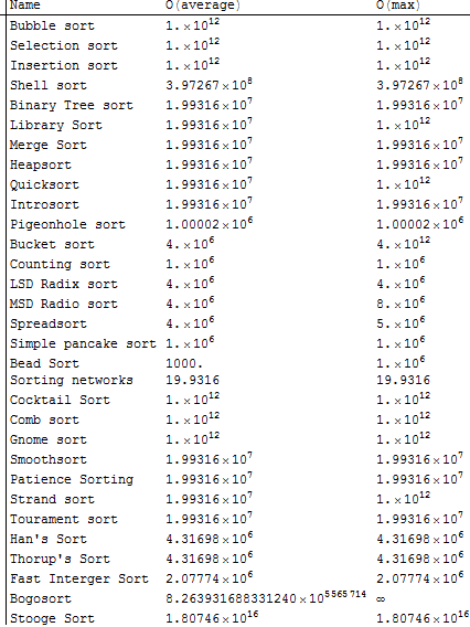
 The complexity of different algorithms in a specific situation.
In this table, n is the number of records to be sorted. The columns "Average" and "Worst" give the time complexity in each case, under the assumption that the length of each key is constant, and that therefore all comparisons, swaps, and other needed operations can proceed in constant time. "Memory" denotes the amount of auxiliary storage needed beyond that used by the list itself, under the same assumption. These are all comparison sorts. The run time and the memory of algorithms could be measured using various notations like theta, sigma, Big-O, small-o, etc. The memory and the run times below are applicable for all the 5 notations.
Comparison sorts Name Best Average Worst Memory Stable Method Other notes Quicksort 


Depends Partitioning Quicksort can be done in place with O(log(n)) stack space, but the sort is unstable[citation needed]. Naïve variants use an O(n) space array to store the partition. An O(n) space implementation can be stable[citation needed]. Merge sort 
Depends Yes Merging Used to sort this table in Firefox [2]. In-place Merge sort 


Yes Merging Implemented in Standard Template Library (STL): [3]; can be implemented as a stable sort based on stable in-place merging: [4] Heapsort No Selection Insertion sort 
Yes Insertion Average case is also  , where d is the number of inversions
Introsort No Partitioning & Selection Used in SGI STL implementations Selection sort Depends [5]. Selection Its stability depends on the implementation. Used to sort this table in Safari or other Webkit web browser [6]. Timsort 
Yes Insertion & Merging comparisons when the data is already sorted or reverse sorted.Shell sort 


depends on gap sequence. Best known: O(nlog 2n) 
No Insertion Bubble sort Yes Exchanging Tiny code size Binary tree sort Yes Insertion When using a self-balancing binary search tree Cycle sort — No Insertion In-place with theoretically optimal number of writes Library sort — Yes Insertion Patience sorting — — No Insertion & Selection Finds all the longest increasing subsequences within O(n log n) Smoothsort No Selection An adaptive sort - comparisons when the data is already sorted, and 0 swaps.Strand sort Yes Selection Tournament sort — Selection Cocktail sort Yes Exchanging Comb sort — — No Exchanging Small code size Gnome sort Yes Exchanging Tiny code size Bogosort 

No Luck Randomly permute the array and check if sorted. The following table describes integer sorting algorithms and other sorting algorithms that are not comparison sorts. As such, they are not limited by a
 lower bound. Complexities below are in terms of n, the number of items to be sorted, k, the size of each key, and d, the digit size used by the implementation. Many of them are based on the assumption that the key size is large enough that all entries have unique key values, and hence that n << 2k, where << means "much less than."
Non-comparison sorts Name Best Average Worst Memory Stable n << 2k Notes Pigeonhole sort — 

Yes Yes Bucket sort (uniform keys) — 


Yes No Assumes uniform distribution of elements from the domain in the array.[2] Bucket sort (integer keys) — 
Yes Yes r is the range of numbers to be sorted. If r =  then Avg RT = [3]
Counting sort — Yes Yes r is the range of numbers to be sorted. If r = then Avg RT = [2]LSD Radix Sort — 
Yes No [3][2] MSD Radix Sort — 
Yes No Stable version uses an external array of size n to hold all of the bins MSD Radix Sort — 
No No In-Place. k / d recursion levels, 2d for count array Spreadsort — 

No No Asymptotics are based on the assumption that n << 2k, but the algorithm does not require this. The following table describes some sorting algorithms that are impractical for real-life use due to extremely poor performance or a requirement for specialized hardware.
Name Best Average Worst Memory Stable Comparison Other notes Bead sort — N/A N/A — N/A No Requires specialized hardware Simple pancake sort — 
No Yes Count is number of flips. Spaghetti (Poll) sort Yes Polling This A linear-time, analog algorithm for sorting a sequence of items, requiring O(n) stack space, and the sort is stable. This requires n parallel processors. Spaghetti sort#Analysis Sorting networks — 
Yes No Requires a custom circuit of size 
Additionally, theoretical computer scientists have detailed other sorting algorithms that provide better than
 time complexity with additional constraints, including:
- Han's algorithm, a deterministic algorithm for sorting keys from a domain of finite size, taking
 time and space.[4]
 - Thorup's algorithm, a randomized algorithm for sorting keys from a domain of finite size, taking time and space.[5]
- An integer sorting algorithm taking
 expected time and space.[6]
Algorithms not yet compared above include:
- Odd-even sort
- Flashsort
- Burstsort
- Postman sort
- Stooge sort
- Samplesort
- Bitonic sorter
- Cocktail sort
- Topological sort
Summaries of popular sorting algorithms
Bubble sort
 A bubble sort, a sorting algorithm that continuously steps through a list, swapping items until they appear in the correct order.Main article: Bubble sort
Bubble sort is a simple sorting algorithm. The algorithm starts at the beginning of the data set. It compares the first two elements, and if the first is greater than the second, it swaps them. It continues doing this for each pair of adjacent elements to the end of the data set. It then starts again with the first two elements, repeating until no swaps have occurred on the last pass. This algorithm's average and worst case performance is O(n2), so it is rarely used to sort large, unordered, data sets. Bubble sort can be used to sort a small number of items (where its inefficiency is not a high penalty). Bubble sort may also be efficiently used on a list that is already sorted except for a very small number of elements. For example, if only one element is not in order, bubble sort will take only 2n time. If two elements are not in order, bubble sort will take only at most 3n time.
Bubble sort average case and worst case are both O(n²).
Selection sort
Main article: Selection sortSelection sort is an in-place comparison sort. It has O(n2) complexity, making it inefficient on large lists, and generally performs worse than the similar insertion sort. Selection sort is noted for its simplicity, and also has performance advantages over more complicated algorithms in certain situations.
The algorithm finds the minimum value, swaps it with the value in the first position, and repeats these steps for the remainder of the list. It does no more than n swaps, and thus is useful where swapping is very expensive.
Insertion sort
Main article: Insertion sortInsertion sort is a simple sorting algorithm that is relatively efficient for small lists and mostly sorted lists, and often is used as part of more sophisticated algorithms. It works by taking elements from the list one by one and inserting them in their correct position into a new sorted list. In arrays, the new list and the remaining elements can share the array's space, but insertion is expensive, requiring shifting all following elements over by one. Shell sort (see below) is a variant of insertion sort that is more efficient for larger lists.
Shell sort
 A Shell sort, different from bubble sort in that it moves elements numerous positions swappingMain article: Shell sort
Shell sort was invented by Donald Shell in 1959. It improves upon bubble sort and insertion sort by moving out of order elements more than one position at a time. One implementation can be described as arranging the data sequence in a two-dimensional array and then sorting the columns of the array using insertion sort.
Comb sort
Main article: Comb sortComb sort is a relatively simplistic sorting algorithm originally designed by Wlodzimierz Dobosiewicz in 1980. Later it was rediscovered and popularized by Stephen Lacey and Richard Box with a Byte Magazine article published in April 1991. Comb sort improves on bubble sort, and rivals algorithms like Quicksort. The basic idea is to eliminate turtles, or small values near the end of the list, since in a bubble sort these slow the sorting down tremendously. (Rabbits, large values around the beginning of the list, do not pose a problem in bubble sort.)
Merge sort
Main article: Merge sortMerge sort takes advantage of the ease of merging already sorted lists into a new sorted list. It starts by comparing every two elements (i.e., 1 with 2, then 3 with 4...) and swapping them if the first should come after the second. It then merges each of the resulting lists of two into lists of four, then merges those lists of four, and so on; until at last two lists are merged into the final sorted list. Of the algorithms described here, this is the first that scales well to very large lists, because its worst-case running time is O(n log n). Merge sort has seen a relatively recent surge in popularity for practical implementations, being used for the standard sort routine in the programming languages Perl,[7] Python (as timsort[8]), and Java (also uses timsort as of JDK7[9]), among others. Merge sort has been used in Java at least since 2000 in JDK1.3.[10][11]
Heapsort
Main article: HeapsortHeapsort is a much more efficient version of selection sort. It also works by determining the largest (or smallest) element of the list, placing that at the end (or beginning) of the list, then continuing with the rest of the list, but accomplishes this task efficiently by using a data structure called a heap, a special type of binary tree. Once the data list has been made into a heap, the root node is guaranteed to be the largest (or smallest) element. When it is removed and placed at the end of the list, the heap is rearranged so the largest element remaining moves to the root. Using the heap, finding the next largest element takes O(log n) time, instead of O(n) for a linear scan as in simple selection sort. This allows Heapsort to run in O(n log n) time, and this is also the worst case complexity.
Quicksort
Main article: QuicksortQuicksort is a divide and conquer algorithm which relies on a partition operation: to partition an array an element called a pivot is selected. All elements smaller than the pivot are moved before it and all greater elements are moved after it. This can be done efficiently in linear time and in-place. The lesser and greater sublists are then recursively sorted. Efficient implementations of quicksort (with in-place partitioning) are typically unstable sorts and somewhat complex, but are among the fastest sorting algorithms in practice. Together with its modest O(log n) space usage, quicksort is one of the most popular sorting algorithms and is available in many standard programming libraries. The most complex issue in quicksort is choosing a good pivot element; consistently poor choices of pivots can result in drastically slower O(n²) performance, if at each step the median is chosen as the pivot then the algorithm works in O(n log n). Finding the median however, is an O(n) operation on unsorted lists and therefore exacts its own penalty with sorting.
Counting sort
Main article: Counting sortCounting sort is applicable when each input is known to belong to a particular set, S, of possibilities. The algorithm runs in O(|S| + n) time and O(|S|) memory where n is the length of the input. It works by creating an integer array of size |S| and using the ith bin to count the occurrences of the ith member of S in the input. Each input is then counted by incrementing the value of its corresponding bin. Afterward, the counting array is looped through to arrange all of the inputs in order. This sorting algorithm cannot often be used because S needs to be reasonably small for it to be efficient, but the algorithm is extremely fast and demonstrates great asymptotic behavior as n increases. It also can be modified to provide stable behavior.
Bucket sort
Main article: Bucket sortBucket sort is a divide and conquer sorting algorithm that generalizes Counting sort by partitioning an array into a finite number of buckets. Each bucket is then sorted individually, either using a different sorting algorithm, or by recursively applying the bucket sorting algorithm. A variation of this method called the single buffered count sort is faster than quicksort.[citation needed]
Due to the fact that bucket sort must use a limited number of buckets it is best suited to be used on data sets of a limited scope. Bucket sort would be unsuitable for data such as social security numbers - which have a lot of variation.
Radix sort
Main article: Radix sortRadix sort is an algorithm that sorts numbers by processing individual digits. n numbers consisting of k digits each are sorted in O(n · k) time. Radix sort can process digits of each number either starting from the least significant digit (LSD) or starting from the most significant digit (MSD). The LSD algorithm first sorts the list by the least significant digit while preserving their relative order using a stable sort. Then it sorts them by the next digit, and so on from the least significant to the most significant, ending up with a sorted list. While the LSD radix sort requires the use of a stable sort, the MSD radix sort algorithm does not (unless stable sorting is desired). In-place MSD radix sort is not stable. It is common for the counting sort algorithm to be used internally by the radix sort. Hybrid sorting approach, such as using insertion sort for small bins improves performance of radix sort significantly.
Distribution sort
Distribution sort refers to any sorting algorithm where data is distributed from its input to multiple intermediate structures which are then gathered and placed on the output. See Bucket sort, Flashsort.
Timsort
Main article: TimsortTimsort finds runs in the data, creates runs with insertion sort if necessary, and then uses merge sort to create the final sorted list. It has the same complexity (O(nlogn)) in the average and worst cases, but with pre-sorted data it goes down to O(n).
Memory usage patterns and index sorting
When the size of the array to be sorted approaches or exceeds the available primary memory, so that (much slower) disk or swap space must be employed, the memory usage pattern of a sorting algorithm becomes important, and an algorithm that might have been fairly efficient when the array fit easily in RAM may become impractical. In this scenario, the total number of comparisons becomes (relatively) less important, and the number of times sections of memory must be copied or swapped to and from the disk can dominate the performance characteristics of an algorithm. Thus, the number of passes and the localization of comparisons can be more important than the raw number of comparisons, since comparisons of nearby elements to one another happen at system bus speed (or, with caching, even at CPU speed), which, compared to disk speed, is virtually instantaneous.
For example, the popular recursive quicksort algorithm provides quite reasonable performance with adequate RAM, but due to the recursive way that it copies portions of the array it becomes much less practical when the array does not fit in RAM, because it may cause a number of slow copy or move operations to and from disk. In that scenario, another algorithm may be preferable even if it requires more total comparisons.
One way to work around this problem, which works well when complex records (such as in a relational database) are being sorted by a relatively small key field, is to create an index into the array and then sort the index, rather than the entire array. (A sorted version of the entire array can then be produced with one pass, reading from the index, but often even that is unnecessary, as having the sorted index is adequate.) Because the index is much smaller than the entire array, it may fit easily in memory where the entire array would not, effectively eliminating the disk-swapping problem. This procedure is sometimes called "tag sort".[12]
Another technique for overcoming the memory-size problem is to combine two algorithms in a way that takes advantages of the strength of each to improve overall performance. For instance, the array might be subdivided into chunks of a size that will fit easily in RAM (say, a few thousand elements), the chunks sorted using an efficient algorithm (such as quicksort or heapsort), and the results merged as per mergesort. This is less efficient than just doing mergesort in the first place, but it requires less physical RAM (to be practical) than a full quicksort on the whole array.
Techniques can also be combined. For sorting very large sets of data that vastly exceed system memory, even the index may need to be sorted using an algorithm or combination of algorithms designed to perform reasonably with virtual memory, i.e., to reduce the amount of swapping required.
Inefficient/humorous sorts
These are algorithms that are extremely slow compared to those discussed above — Bogosort
 , Stooge sort O(n2.7).
See also
- External sorting
- Sorting networks (compare)
- Cocktail sort
- Collation
- Schwartzian transform
- Shuffling algorithms
- Search algorithms
References
- ^ Demuth, H. Electronic Data Sorting. PhD thesis, Stanford University, 1956.
- ^ a b c Cormen, Thomas H.; Leiserson, Charles E., Rivest, Ronald L., Stein, Clifford (2001) [1990]. Introduction to Algorithms (2nd ed.). MIT Press and McGraw-Hill. ISBN 0-262-03293-7.
- ^ a b Goodrich, Michael T.; Tamassia, Roberto (2002). "4.5 Bucket-Sort and Radix-Sort". Algorithm Design: Foundations, Analysis, and Internet Examples. John Wiley & Sons. pp. 241–243.
- ^ Y. Han. Deterministic sorting in time and linear space. Proceedings of the thirty-fourth annual ACM symposium on Theory of computing, Montreal, Quebec, Canada, 2002,p.602-608.
- ^ M. Thorup. Randomized Sorting in Time and Linear Space Using Addition, Shift, and Bit-wise Boolean Operations. Journal of Algorithms, Volume 42, Number 2, February 2002, pp. 205-230(26)
- ^ Han, Y. and Thorup, M. 2002. Integer Sorting in Expected Time and Linear Space. In Proceedings of the 43rd Symposium on Foundations of Computer Science (November 16–19, 2002). FOCS. IEEE Computer Society, Washington, DC, 135-144.
- ^ Perl sort documentation
- ^ Tim Peters's original description of timsort
- ^ [1]
- ^ Merge sort in Java 1.3, Sun.
- ^ Java 1.3 live since 2000
- ^ Definition of "tag sort" according to PC Magazine
- D. E. Knuth, The Art of Computer Programming, Volume 3: Sorting and Searching.
External links
- Sorting Algorithm Animations - Graphical illustration of how different algorithms handle different kinds of data sets.
- Sequential and parallel sorting algorithms - Explanations and analyses of many sorting algorithms.
- Dictionary of Algorithms, Data Structures, and Problems - Dictionary of algorithms, techniques, common functions, and problems.
- Slightly Skeptical View on Sorting Algorithms Discusses several classic algorithms and promotes alternatives to the quicksort algorithm.
Sorting algorithms Theory Exchange sorts Selection sorts - Selection sort
- Heapsort
- Smoothsort
- Cartesian tree sort
- Tournament sort
- Cycle sort
Insertion sorts Merge sorts Distribution sorts Concurrent sorts - Bitonic sorter
- Batcher odd–even mergesort
- Pairwise sorting network
Hybrid sorts - Timsort
- Introsort
- Spreadsort
- UnShuffle sort
- JSort
Quantum sorts Other Categories:- Sorting algorithms


Wikimedia Foundation. 2010.