Travelling salesman problem

The travelling salesman problem (TSP) is an NP-hard problem in combinatorial optimization studied in operations research and theoretical computer science. Given a list of cities and their pairwise distances, the task is to find a shortest possible tour that visits each city exactly once. It is a special case of the Traveling purchaser problem.

The problem was first formulated as a mathematical problem in 1930 and is one of the most intensively studied problems in optimization. It is used as a benchmark for many optimization methods. Even though the problem is computationally difficult, a large number of heuristics and exact methods are known, so that some instances with tens of thousands of cities can be solved.

The TSP has several applications even in its purest formulation, such as planning, logistics, and the manufacture of microchips. Slightly modified, it appears as a sub-problem in many areas, such as DNA sequencing. In these applications, the concept city represents, for example, customers, soldering points, or DNA fragments, and the concept distance represents travelling times or cost, or a similarity measure between DNA fragments. In many applications, additional constraints such as limited resources or time windows make the problem considerably harder.

In the theory of computational complexity, the decision version of the TSP (where, given a length L, the task is to decide whether any tour is shorter than L) belongs to the class of NP-complete problems. Thus, it is likely that the worst case running time for any algorithm for the TSP increases exponentially with the number of cities.

History

The origins of the travelling salesman problem are unclear. A handbook for travelling salesmen from 1832 mentions the problem and includes example tours through Germany and Switzerland, but contains no mathematical treatment.^[1]

William Rowan Hamilton

The travelling salesman problem was defined in the 1800s by the Irish mathematician W. R. Hamilton and by the British mathematician Thomas Kirkman. Hamilton’s Icosian Game was a recreational puzzle based on finding a Hamiltonian cycle.^[2] The general form of the TSP appears to have been first studied by mathematicians during the 1930s in Vienna and at Harvard, notably by Karl Menger, who defines the problem, considers the obvious brute-force algorithm, and observes the non-optimality of the nearest neighbour heuristic:

We denote by messenger problem (since in practice this question should be solved by each postman, anyway also by many travelers) the task to find, for ﬁnitely many points whose pairwise distances are known, the shortest route connecting the points. Of course, this problem is solvable by finitely many trials. Rules which would push the number of trials below the number of permutations of the given points, are not known. The rule that one first should go from the starting point to the closest point, then to the point closest to this, etc., in general does not yield the shortest route.^[3]

Hassler Whitney at Princeton University introduced the name travelling salesman problem soon after.^[4]

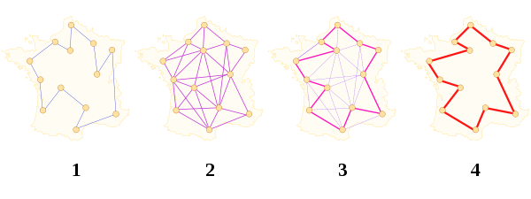
In the 1950s and 1960s, the problem became increasingly popular in scientific circles in Europe and the USA. Notable contributions were made by George Dantzig, Delbert Ray Fulkerson and Selmer M. Johnson at the RAND Corporation in Santa Monica, who expressed the problem as an integer linear program and developed the cutting plane method for its solution. With these new methods they solved an instance with 49 cities to optimality by constructing a tour and proving that no other tour could be shorter. In the following decades, the problem was studied by many researchers from mathematics, computer science, chemistry, physics, and other sciences.

Richard M. Karp showed in 1972 that the Hamiltonian cycle problem was NP-complete, which implies the NP-hardness of TSP. This supplied a mathematical explanation for the apparent computational difficulty of finding optimal tours.

Great progress was made in the late 1970s and 1980, when Grötschel, Padberg, Rinaldi and others managed to exactly solve instances with up to 2392 cities, using cutting planes and branch-and-bound.

In the 1990s, Applegate, Bixby, Chvátal, and Cook developed the program Concorde that has been used in many recent record solutions. Gerhard Reinelt published the TSPLIB in 1991, a collection of benchmark instances of varying difficulty, which has been used by many research groups for comparing results. In 2005, Cook and others computed an optimal tour through a 33,810-city instance given by a microchip layout problem, currently the largest solved TSPLIB instance. For many other instances with millions of cities, solutions can be found that are guaranteed to be within 1% of an optimal tour.^{[citation needed]}

Description

As a graph problem

Symmetric TSP with four cities

TSP can be modeled as an undirected weighted graph, such that cities are the graph's vertices, paths are the graph's edges, and a path's distance is the edge's length. A TSP tour becomes a Hamiltonian cycle if and only if every edge has the same distance. Often, the model is a complete graph (i.e., an edge connects each pair of vertices). If no path exists between two cities, adding an arbitrarily long edge will complete the graph without affecting the optimal tour.

Asymmetric and symmetric

In the symmetric TSP, the distance between two cities is the same in each opposite direction, forming an undirected graph. This symmetry halves the number of possible solutions. In the asymmetric TSP, paths may not exist in both directions or the distances might be different, forming a directed graph. Traffic collisions, one-way streets, and airfares for cities with different departure and arrival fees are examples of how this symmetry could break down.

Computing a solution

The traditional lines of attack for the NP-hard problems are the following:

Devising algorithms for finding exact solutions (they will work reasonably fast only for small problem sizes).
Devising "suboptimal" or heuristic algorithms, i.e., algorithms that deliver either seemingly or probably good solutions, but which could not be proved to be optimal.
Finding special cases for the problem ("subproblems") for which either better or exact heuristics are possible.

Computational complexity

The problem has been shown to be NP-hard (more precisely, it is complete for the complexity class FP^NP; see function problem), and the decision problem version ("given the costs and a number x, decide whether there is a round-trip route cheaper than x") is NP-complete. The bottleneck travelling salesman problem is also NP-hard. The problem remains NP-hard even for the case when the cities are in the plane with Euclidean distances, as well as in a number of other restrictive cases. Removing the condition of visiting each city "only once" does not remove the NP-hardness, since it is easily seen that in the planar case there is an optimal tour that visits each city only once (otherwise, by the triangle inequality, a shortcut that skips a repeated visit would not increase the tour length).

Complexity of approximation

In the general case, finding a shortest travelling salesman tour is NPO-complete.^[6] If the distance measure is a metric and symmetric, the problem becomes APX-complete^[7] and Christofides’s algorithm approximates it within 1.5.^[8]

If the distances are restricted to 1 and 2 (but still are a metric) the approximation ratio becomes 7/6. In the asymmetric, metric case, only logarithmic performance guarantees are known, the best current algorithm achieves performance ratio 0.814 log n;^[9] it is an open question if a constant factor approximation exists.

The corresponding maximization problem of finding the longest travelling salesman tour is approximable within 63/38.^[10] If the distance function is symmetric, the longest tour can be approximated within 4/3 by a deterministic algorithm^[11] and within $(33+\epsilon)/25$ by a randomised algorithm.^[12]

Exact algorithms

The most direct solution would be to try all permutations (ordered combinations) and see which one is cheapest (using brute force search). The running time for this approach lies within a polynomial factor of O(n!), the factorial of the number of cities, so this solution becomes impractical even for only 20 cities. One of the earliest applications of dynamic programming is the Held–Karp algorithm that solves the problem in time O(n²2ⁿ).^[13]

The dynamic programming solution requires exponential space. Using inclusion–exclusion, the problem can be solved in time within a polynomial factor of $2 n$ and polynomial space.^[14]

Improving these time bounds seems to be difficult. For example, it has not been determined whether an exact algorithm for TSP that runs in time $O (1.9999 n)$ exists.^[15]

Other approaches include:

Various branch-and-bound algorithms, which can be used to process TSPs containing 40–60 cities.
Progressive improvement algorithms which use techniques reminiscent of linear programming. Works well for up to 200 cities.
Implementations of branch-and-bound and problem-specific cut generation; this is the method of choice for solving large instances. This approach holds the current record, solving an instance with 85,900 cities, see Applegate et al. (2006).

An exact solution for 15,112 German towns from TSPLIB was found in 2001 using the cutting-plane method proposed by George Dantzig, Ray Fulkerson, and Selmer M. Johnson in 1954, based on linear programming. The computations were performed on a network of 110 processors located at Rice University and Princeton University (see the Princeton external link). The total computation time was equivalent to 22.6 years on a single 500 MHz Alpha processor. In May 2004, the travelling salesman problem of visiting all 24,978 towns in Sweden was solved: a tour of length approximately 72,500 kilometers was found and it was proven that no shorter tour exists.^[16]

In March 2005, the travelling salesman problem of visiting all 33,810 points in a circuit board was solved using Concorde TSP Solver: a tour of length 66,048,945 units was found and it was proven that no shorter tour exists. The computation took approximately 15.7 CPU-years (Cook et al. 2006). In April 2006 an instance with 85,900 points was solved using Concorde TSP Solver, taking over 136 CPU-years, see Applegate et al. (2006).

Heuristic and approximation algorithms

Various heuristics and approximation algorithms, which quickly yield good solutions have been devised. Modern methods can find solutions for extremely large problems (millions of cities) within a reasonable time which are with a high probability just 2–3% away from the optimal solution.

Several categories of heuristics are recognized.

Constructive heuristics

The nearest neighbour (NN) algorithm (or so-called greedy algorithm) lets the salesman choose the nearest unvisited city as his next move. This algorithm quickly yields an effectively short route. For N cities randomly distributed on a plane, the algorithm on average yields a path 25% longer than the shortest possible path.^[17] However, there exist many specially arranged city distributions which make the NN algorithm give the worst route (Gutin, Yeo, and Zverovich, 2002). This is true for both asymmetric and symmetric TSPs (Gutin and Yeo, 2007). Rosenkrantz et al. [1977] showed that the NN algorithm has the approximation factor $Θ(log | V | )$ for instances satisfying the triangle inequality.

Constructions based on a minimum spanning tree have an approximation ratio of 2. The Christofides algorithm achieves a ratio of 1.5.

The bitonic tour of a set of points is the minimum-perimeter monotone polygon that has the points as its vertices; it can be computed efficiently by dynamic programming.

Another constructive heuristic, Match Twice and Stitch (MTS) (Kahng, Reda 2004 ^[18]), performs two sequential matchings, where the second matching is executed after deleting all the edges of the first matching, to yield a set of cycles. The cycles are then stitched to produce the final tour.

Iterative improvement

Pairwise exchange, or Lin–Kernighan heuristics: The pairwise exchange or 2-opt technique involves iteratively removing two edges and replacing these with two different edges that reconnect the fragments created by edge removal into a new and shorter tour. This is a special case of the k-opt method. Note that the label Lin–Kernighan is an often heard misnomer for 2-opt. Lin–Kernighan is actually a more general method.
k-opt heuristic: Take a given tour and delete k mutually disjoint edges. Reassemble the remaining fragments into a tour, leaving no disjoint subtours (that is, don't connect a fragment's endpoints together). This in effect simplifies the TSP under consideration into a much simpler problem. Each fragment endpoint can be connected to 2k − 2 other possibilities: of 2k total fragment endpoints available, the two endpoints of the fragment under consideration are disallowed. Such a constrained 2k-city TSP can then be solved with brute force methods to find the least-cost recombination of the original fragments. The k-opt technique is a special case of the V-opt or variable-opt technique. The most popular of the k-opt methods are 3-opt, and these were introduced by Shen Lin of Bell Labs in 1965. There is a special case of 3-opt where the edges are not disjoint (two of the edges are adjacent to one another). In practice, it is often possible to achieve substantial improvement over 2-opt without the combinatorial cost of the general 3-opt by restricting the 3-changes to this special subset where two of the removed edges are adjacent. This so-called two-and-a-half-opt typically falls roughly midway between 2-opt and 3-opt, both in terms of the quality of tours achieved and the time required to achieve those tours.
V-opt heuristic: The variable-opt method is related to, and a generalization of the k-opt method. Whereas the k-opt methods remove a fixed number (k) of edges from the original tour, the variable-opt methods do not fix the size of the edge set to remove. Instead they grow the set as the search process continues. The best known method in this family is the Lin–Kernighan method (mentioned above as a misnomer for 2-opt). Shen Lin and Brian Kernighan first published their method in 1972, and it was the most reliable heuristic for solving travelling salesman problems for nearly two decades. More advanced variable-opt methods were developed at Bell Labs in the late 1980s by David Johnson and his research team. These methods (sometimes called Lin–Kernighan–Johnson) build on the Lin–Kernighan method, adding ideas from tabu search and evolutionary computing. The basic Lin–Kernighan technique gives results that are guaranteed to be at least 3-opt. The Lin–Kernighan–Johnson methods compute a Lin–Kernighan tour, and then perturb the tour by what has been described as a mutation that removes at least four edges and reconnecting the tour in a different way, then v-opting the new tour. The mutation is often enough to move the tour from the local minimum identified by Lin–Kernighan. V-opt methods are widely considered the most powerful heuristics for the problem, and are able to address special cases, such as the Hamilton Cycle Problem and other non-metric TSPs that other heuristics fail on. For many years Lin–Kernighan–Johnson had identified optimal solutions for all TSPs where an optimal solution was known and had identified the best known solutions for all other TSPs on which the method had been tried.

Randomised improvement

Optimized Markov chain algorithms which use local searching heuristic sub-algorithms can find a route extremely close to the optimal route for 700 to 800 cities.

TSP is a touchstone for many general heuristics devised for combinatorial optimization such as genetic algorithms, simulated annealing, Tabu search, ant colony optimization, river formation dynamics (see swarm intelligence) and the cross entropy method.

Ant colony optimization

Artificial intelligence researcher Marco Dorigo described in 1997 a method of heuristically generating "good solutions" to the TSP using a simulation of an ant colony called ACS (Ant Colony System).^[19] It models behavior observed in real ants to find short paths between food sources and their nest, an emergent behaviour resulting from each ant's preference to follow trail pheromones deposited by other ants.

ACS sends out a large number of virtual ant agents to explore many possible routes on the map. Each ant probabilistically chooses the next city to visit based on a heuristic combining the distance to the city and the amount of virtual pheromone deposited on the edge to the city. The ants explore, depositing pheromone on each edge that they cross, until they have all completed a tour. At this point the ant which completed the shortest tour deposits virtual pheromone along its complete tour route (global trail updating). The amount of pheromone deposited is inversely proportional to the tour length: the shorter the tour, the more it deposits.

Special cases

Metric TSP

In the metric TSP, also known as delta-TSP or Δ-TSP, the intercity distances satisfy the triangle inequality.

A very natural restriction of the TSP is to require that the distances between cities form a metric, i.e., they satisfy the triangle inequality. This can be understood as the absence of "shortcuts", in the sense that the direct connection from A to B is never longer than the route via intermediate C:

$d_{AB} \le d_{AC} + d_{CB}$

The edge lengths then form a metric on the set of vertices. When the cities are viewed as points in the plane, many natural distance functions are metrics, and so many natural instances of TSP satisfy this constraint.

The following are some examples of metric TSPs for various metrics.

In the Euclidean TSP (see below) the distance between two cities is the Euclidean distance between the corresponding points.
In the rectilinear TSP the distance between two cities is the sum of the differences of their x- and y-coordinates. This metric is often called the Manhattan distance or city-block metric.
In the maximum metric, the distance between two points is the maximum of the absolute values of differences of their x- and y-coordinates.

The last two metrics appear for example in routing a machine that drills a given set of holes in a printed circuit board. The Manhattan metric corresponds to a machine that adjusts first one co-ordinate, and then the other, so the time to move to a new point is the sum of both movements. The maximum metric corresponds to a machine that adjusts both co-ordinates simultaneously, so the time to move to a new point is the slower of the two movements.

In its definition, the TSP does not allow cities to be visited twice, but many applications do not need this constraint. In such cases, a symmetric, non-metric instance can be reduced to a metric one. This replaces the original graph with a complete graph in which the inter-city distance $d A B$ is replaced by the shortest path between $A$ and $B$ in the original graph.

There is a constant-factor approximation algorithm for the metric TSP due to Christofides^[20] that always finds a tour of length at most 1.5 times the shortest tour. In the next paragraphs, we explain a weaker (but simpler) algorithm which finds a tour of length at most twice the shortest tour.

The length of the minimum spanning tree of the network is a natural lower bound for the length of the optimal route. In the TSP with triangle inequality case it is possible to prove upper bounds in terms of the minimum spanning tree and design an algorithm that has a provable upper bound on the length of the route. The first published (and the simplest) example follows:

Construct the minimum spanning tree.
Duplicate all its edges. That is, wherever there is an edge from u to v, add a second edge from u to v. This gives us an Eulerian graph.
Find a Eulerian cycle in it. Clearly, its length is twice the length of the tree.
Convert the Eulerian cycle into the Hamiltonian one in the following way: walk along the Eulerian cycle, and each time you are about to come into an already visited vertex, skip it and try to go to the next one (along the Eulerian cycle).

It is easy to prove that the last step works. Moreover, thanks to the triangle inequality, each skipping at Step 4 is in fact a shortcut; i.e., the length of the cycle does not increase. Hence it gives us a TSP tour no more than twice as long as the optimal one.

The Christofides algorithm follows a similar outline but combines the minimum spanning tree with a solution of another problem, minimum-weight perfect matching. This gives a TSP tour which is at most 1.5 times the optimal. The Christofides algorithm was one of the first approximation algorithms, and was in part responsible for drawing attention to approximation algorithms as a practical approach to intractable problems. As a matter of fact, the term "algorithm" was not commonly extended to approximation algorithms until later; the Christofides algorithm was initially referred to as the Christofides heuristic.

In the special case that distances between cities are all either one or two (and thus the triangle inequality is necessarily satisfied), there is a polynomial-time approximation algorithm that finds a tour of length at most 8/7 times the optimal tour length.^[21] However, it is a long-standing (since 1975) open problem to improve the Christofides approximation factor of 1.5 for general metric TSP to a smaller constant. It is known that, unless P = NP, there is no polynomial-time algorithm that finds a tour of length at most 220/219=1.00456… times the optimal tour's length.^[22] In the case of bounded metrics it is known that there is no polynomial time algorithm that constructs a tour of length at most 321/320 times the optimal tour's length, unless P = NP.^[23]

Euclidean TSP

The Euclidean TSP, or planar TSP, is the TSP with the distance being the ordinary Euclidean distance.

The Euclidean TSP is a particular case of the metric TSP, since distances in a plane obey the triangle inequality.

Like the general TSP, the Euclidean TSP (and therefore the general metric TSP) is NP-complete.^[24] However, in some respects it seems to be easier than the general metric TSP. For example, the minimum spanning tree of the graph associated with an instance of the Euclidean TSP is a Euclidean minimum spanning tree, and so can be computed in expected O(n log n) time for n points (considerably less than the number of edges). This enables the simple 2-approximation algorithm for TSP with triangle inequality above to operate more quickly.

In general, for any c > 0, where d is the number of dimensions in the Euclidean space, there is a polynomial-time algorithm that finds a tour of length at most (1 + 1/c) times the optimal for geometric instances of TSP in $O\left(n (\log n)^{(O(c \sqrt{d}))^{d-1}}\right)$ time; this is called a polynomial-time approximation scheme (PTAS).^[25] Sanjeev Arora and Joseph S. B. Mitchell were awarded the Gödel Prize for their concurrent discovery of a PTAS for the Euclidean TSP in 2010.

In practice, heuristics with weaker guarantees continue to be used.

Asymmetric TSP

In most cases, the distance between two nodes in the TSP network is the same in both directions. The case where the distance from A to B is not equal to the distance from B to A is called asymmetric TSP. A practical application of an asymmetric TSP is route optimisation using street-level routing (which is made asymmetric by one-way streets, slip-roads, motorways, etc.).

Solving by conversion to symmetric TSP

Solving an asymmetric TSP graph can be somewhat complex. The following is a 3×3 matrix containing all possible path weights between the nodes A, B and C. One option is to turn an asymmetric matrix of size N into a symmetric matrix of size 2N.^[26]

Asymmetric path weights
	A	B	C
A		1	2
B	6		3
C	5	4

To double the size, each of the nodes in the graph is duplicated, creating a second ghost node. Using duplicate points with very low weights, such as −∞, provides a cheap route "linking" back to the real node and allowing symmetric evaluation to continue. The original 3×3 matrix shown above is visible in the bottom left and the inverse of the original in the top-right. Both copies of the matrix have had their diagonals replaced by the low-cost hop paths, represented by −∞.

Symmetric path weights
	A	B	C	A′	B′	C′
A				−∞	6	5
B				1	−∞	4
C				2	3	−∞
A′	−∞	1	2
B′	6	−∞	3
C′	5	4	−∞

The original 3×3 matrix would produce two Hamiltonian cycles (a path that visits every node once), namely A-B-C-A [score 9] and A-C-B-A [score 12]. Evaluating the 6×6 symmetric version of the same problem now produces many paths, including A-A′-B-B′-C-C′-A, A-B′-C-A′-A, A-A′-B-C′-A [all score 9 – ∞].

The important thing about each new sequence is that there will be an alternation between dashed (A′,B′,C′) and un-dashed nodes (A, B, C) and that the link to "jump" between any related pair (A-A′) is effectively free. A version of the algorithm could use any weight for the A-A′ path, as long as that weight is lower than all other path weights present in the graph. As the path weight to "jump" must effectively be "free", the value zero (0) could be used to represent this cost—if zero is not being used for another purpose already (such as designating invalid paths). In the two examples above, non-existent paths between nodes are shown as a blank square.

Benchmarks

For benchmarking of TSP algorithms, TSPLIB is a library of sample instances of the TSP and related problems is maintained, see the TSPLIB external reference. Many of them are lists of actual cities and layouts of actual printed circuits.

Human performance on TSP

The TSP, in particular the Euclidean variant of the problem, has attracted the attention of researchers in cognitive psychology. It is observed that humans are able to produce good quality solutions quickly. The first issue of the Journal of Problem Solving is devoted to the topic of human performance on TSP.

TSP path length for random pointset in a square

Suppose N points are randomly distributed in a 1 x 1 square with N>>1. Consider many such squares. Suppose we want to know the average of the shortest path length (i.e. TSP solution) of each square.

Lower bound

$\frac{1}{2} \sqrt{N}$ is a lower bound obtained by assuming i be a point in the tour sequence and i has its nearest neighbor as its next in the path.

$\left({\frac{1}{4} + \frac{3}{8}}\right)\sqrt{N}$ is a better lower bound obtained by assuming is next is is nearest, and is previous is is second nearest.

$\sqrt{\frac{N}{2}}$ is an even better lower bound obtained by dividing the path sequence into two parts as before_i and after_i with each part containing N/2 points, and then deleting the before_i part to form a diluted pointset (see discussion).

David S. Johnson^[27] obtained a lower bound by computer experiment:

$0.7080\sqrt{N}+0.522$ , where 0.522 comes from the points near square boundary which have fewer neighbors.

Christine L. Valenzuela and Antonia J. Jones ^[28] obtained another lower bound by computer experiment:

$0.7078\sqrt{N}+0.551$

Upper bound

By applying Simulated Annealing method on samples of N=40000, computer analysis shows an upper bound of

$\left(\sqrt{\frac{N}{2}}+0.72\right) \cdot 1.015$ , where 0.72 comes from the boundary effect.

Because the actual solution is only the shortest path, for the purposes of programmatic search another upper bound is the length of any previously discovered approximation.

Analyst's traveling salesman problem

There is an analogous problem in geometric measure theory which asks the following: under what conditions may a subset E of Euclidean space be contained in a rectifiable curve (that is, when is there a continuous curve that visits every point in E)? This problem is known as the analyst's traveling salesman problem or the geometric traveling salesman problem.

Notes

^ “Der Handlungsreisende – wie er sein soll und was er zu thun [sic] hat, um Aufträge zu erhalten und eines glücklichen Erfolgs in seinen Geschäften gewiß zu sein – von einem alten Commis-Voyageur” (The traveling salesman — how he must be and what he should do in order to be sure to perform his tasks and have success in his business — by a high commis-voyageur)
^ A discussion of the early work of Hamilton and Kirkman can be found in Graph Theory 1736–1936
^ Cited and English translation in Schrijver (2005). Original German: “Wir bezeichnen als Botenproblem (weil diese Frage in der Praxis von jedem Postboten, übrigens auch von vielen Reisenden zu lösen ist) die Aufgabe, für endlich viele Punkte, deren paarweise Abstände bekannt sind, den kürzesten die Punkte verbindenden Weg zu finden. Dieses Problem ist natürlich stets durch endlich viele Versuche lösbar. Regeln, welche die Anzahl der Versuche unter die Anzahl der Permutationen der gegebenen Punkte herunterdrücken würden, sind nicht bekannt. Die Regel, man solle vom Ausgangspunkt erst zum nächstgelegenen Punkt, dann zu dem diesem nächstgelegenen Punkt gehen usw., liefert im allgemeinen nicht den kürzesten Weg.”
^ A detailed treatment of the connection between Menger and Whitney as well as the growth in the study of TSP can be found in Alexander Schrijver's 2005 paper "On the history of combinatorial optimization (till 1960). Handbook of Discrete Optimization (K. Aardal, G.L. Nemhauser, R. Weismantel, eds.), Elsevier, Amsterdam, 2005, pp. 1–68.PS,PDF
^ Behzad, Arash; Modarres, Mohammad (2002), "New Efficient Transformation of the Generalized Traveling Salesman Problem into Traveling Salesman Problem", Proceedings of the 15th International Conference of Systems Engineering (Las Vegas)
^ Orponen (1987)
^ Papadimitriou (1983)
^ Christofides (1976)
^ Kaplan (2004)
^ Kosaraju (1994)
^ Serdyukov (1984)
^ Hassin (2000)
^ Bellman (1960), Bellman (1962), Held & Karp (1962)
^ Kohn (1977) Karp (1982)
^ Woeginger (2003)
^ Work by David Applegate, AT&T Labs – Research, Robert Bixby, ILOG and Rice University, Vašek Chvátal, Concordia University, William Cook, Georgia Tech, and Keld Helsgaun, Roskilde University is discussed on their project web page hosted by Georgia Tech and last updated in June 2004, here [1]
^ Johnson, D.S. and McGeoch, L.A.. "The traveling salesman problem: A case study in local optimization", Local search in combinatorial optimization, 1997, 215-310
^ A. B. Kahng and S. Reda, "Match Twice and Stitch: A New TSP Tour Construction Heuristic," Operations Research Letters, 2004, 32(6). pp. 499–509. http://dx.doi.org/10.1016/j.orl.2004.04.001
^ Marco Dorigo. Ant Colonies for the Traveling Salesman Problem. IRIDIA, Université Libre de Bruxelles. IEEE Transactions on Evolutionary Computation, 1(1):53–66. 1997. http://citeseer.ist.psu.edu/86357.html
^ N. Christofides, Worst-case analysis of a new heuristic for the traveling salesman problem, Report 388, Graduate School of Industrial Administration, Carnegie Mellon University, 1976.
^ P. Berman (2006). M. Karpinski, "8/7-Approximation Algorithm for (1,2)-TSP", Proc. 17th ACM-SIAM SODA (2006), pp. 641–648, ECCC TR05-069.
^ C.H. Papadimitriou and Santosh Vempala. On the approximability of the traveling salesman problem, Combinatorica 26(1):101–120, 2006.
^ L. Engebretsen, M. Karpinski, TSP with bounded metrics. Journal of Computer and System Sciences, 72(4):509‒546, 2006.
^ Christos H. Papadimitriou. "The Euclidean travelling salesman problem is NP-complete". Theoretical Computer Science 4:237–244, 1977. doi:10.1016/0304-3975(77)90012-3
^ Sanjeev Arora. Polynomial Time Approximation Schemes for Euclidean Traveling Salesman and other Geometric Problems. Journal of the ACM, Vol.45, Issue 5, pp.753–782. ISSN:0004-5411. September 1998. http://citeseer.ist.psu.edu/arora96polynomial.html.
^ Roy Jonker, Ton Volgenant, Transforming asymmetric into symmetric traveling salesman problems , Operations Research Letters, Volume 2, Issue 4, November 1983, Pages 161-163, ISSN 0167-6377, DOI: 10.1016/0167-6377(83)90048-2.
^ David S. Johnson
^ Christine L. Valenzuela and Antonia J. Jones

References

Applegate, D. L.; Bixby, R. M.; Chvátal, V.; Cook, W. J. (2006), The Traveling Salesman Problem, ISBN 0691129932 .
Bellman, R. (1960), "Combinatorial Processes and Dynamic Programming", in Bellman, R., Hall, M., Jr. (eds.), Combinatorial Analysis, Proceedings of Symposia in Applied Mathematics 10,, American Mathematical Society, pp. 217–249 .
Bellman, R. (1962), "Dynamic Programming Treatment of the Travelling Salesman Problem", J. Assoc. Comput. Mach. 9: 61–63, doi:10.1145/321105.321111 .
Christofides, N. (1976), Worst-case analysis of a new heuristic for the travelling salesman problem, Technical Report 388, Graduate School of Industrial Administration, Carnegie-Mellon University, Pittsburgh .
Hassin, R.; Rubinstein, S. (2000), "Better approximations for max TSP", Information Processing Letters 75 (4): 181–186, doi:10.1016/S0020-0190(00)00097-1 .
Held, M.; Karp, R. M. (1962), "A Dynamic Programming Approach to Sequencing Problems", Journal of the Society for Industrial and Applied Mathematics 10 (1): 196–210, doi:10.1137/0110015 .
Kaplan, H.; Lewenstein, L.; Shafrir, N.; Sviridenko, M. (2004), "Approximation Algorithms for Asymmetric TSP by Decomposing Directed Regular Multigraphs", In Proc. 44th IEEE Symp. on Foundations of Comput. Sci, pp. 56–65 .
Karp, R.M. (1982), "Dynamic programming meets the principle of inclusion and exclusion", Oper. Res. Lett. 1 (2): 49–51, doi:10.1016/0167-6377(82)90044-X .
Kohn, S.; Gottlieb, A.; Kohn, M. (1977), "A Generating Function Approach to the Traveling Salesman Problem", ACM Annual Conference, ACM Press, pp. 294–300 .
Kosaraju, S. R.; Park, J. K.; Stein, C. (1994), "Long tours and short superstrings'", Proc. 35th Ann. IEEE Symp. on Foundations of Comput. Sci, IEEE Computer Society, pp. 166–177 .
Orponen, P.; Mannila, H. (1987), "On approximation preserving reductions: Complete problems and robust measures'", Technical Report C-1987–28, Department of Computer Science, University of Helsinki .
Papadimitriou, C. H.; Yannakakis, M. (1993), "The traveling salesman problem with distances one and two", Math. Oper. Res. 18: 1–11, doi:10.1287/moor.18.1.1 .
Serdyukov, A. I. (1984), "An algorithm with an estimate for the traveling salesman problem of the maximum'", Upravlyaemye Sistemy 25: 80–86 .
Woeginger, G.J. (2003), "Exact Algorithms for NP-Hard Problems: A Survey", Combinatorial Optimization – Eureka, You Shrink! Lecture notes in computer science, vol. 2570, Springer, pp. 185–207 .

External links

Traveling Salesman Problem at Georgia Tech
TSPLIB at the University of Heidelberg
Traveling Salesman Problem by Jon McLoone based on a program by Stephen Wolfram, after work by Stan Wagon, Wolfram Demonstrations Project.
optimap an approximation using ACO on GoogleMaps with JavaScript
tsp an exact solver using Constraint Programming on GoogleMaps
Demo applet of a genetic algorithm solving TSPs and VRPTW problems
Source code library for the travelling salesman problem
TSP solvers in R for symmetric and asymmetric TSPs. Implements various insertion, nearest neighbor and 2-opt heuristics and an interface to Georgia Tech's Concorde and Chained Lin-Kernighan heuristics.

Categories:

Travelling salesman problem
NP-complete problems
Operations research
Graph algorithms
Computational problems in graph theory

Wikimedia Foundation. 2010.

Игры ⚽ Поможем сделать НИР

Look at other dictionaries:

Travelling Salesman Problem — [ trævəlɪȖ seɪlzmən prɔbləm, englisch], Problem des Handelsreisenden, Rundfahrtproblem, Operations Research: kombinatorisches Optimierungsproblem, bei dem durch eine vorgegebene Menge von Orten von einem bestimmten Ausgangsort aus der kürzeste… … Universal-Lexikon
Travelling-Salesman-Problem — Optimaler Reiseweg eines Handlungsreisenden durch die 15 größten Städte Deutschlands. Die angegebene Route ist die kürzeste von 43.589.145.600 möglichen. Das Problem des Handlungsreisenden (engl. Traveling Salesman Problem, kurz TSP) ist ein … Deutsch Wikipedia
Travelling Salesman Problem — Optimaler Reiseweg eines Handlungsreisenden durch die 15 größten Städte Deutschlands. Die angegebene Route ist die kürzeste von 43.589.145.600 möglichen. Das Problem des Handlungsreisenden (engl. Traveling Salesman Problem, kurz TSP) ist ein … Deutsch Wikipedia
travelling salesman problem — noun The problem in combinatorial optimization in which, given a number of cities and the costs of travelling from one to the other, it is required to determine the cheapest route that visits each city once and then returns to the initial city … Wiktionary
Travelling salesman (disambiguation) — A travelling salesman is a travelling vendor of goods.Travelling salesman may also refer to:* Traveling Saleseman (film), a 1921 comedy film * Traveling Salesmen ( The Office episode), the twelfth episode of the third season of the US version of… … Wikipedia
Bottleneck traveling salesman problem — The Bottleneck traveling salesman problem (bottleneck TSP) is a problem in discrete or combinatorial optimization. It is stated as follows: Find the Hamiltonian cycle in a weighted graph with the minimal weight of the most weighty edge of the… … Wikipedia
Function problem — In computational complexity theory, a function problem is a problem other than a decision problem, that is, a problem requiring a more complex answer than just YES or NO.Notable examples include the travelling salesman problem, which asks for the … Wikipedia
P versus NP problem — Unsolved problems in computer science Is P = NP ? … Wikipedia
Job-shop problem — The job shop problem (JSP) is a problem in discrete or combinatorial optimization, and is a generalization of the famous travelling salesman problem. It is a prominent illustration of a class of problems in computational complexity theory which… … Wikipedia
P = NP problem — The relationship between the complexity classes P and NP is an unsolved question in theoretical computer science. It is considered to be the most important problem in the field – the Clay Mathematics Institute has offered a $1 million US prize… … Wikipedia

Academic Dictionaries and Encyclopedias

Travelling salesman problem

Contents

History