- Morse theory
-
- "Morse function" redirects here. In another context, a "Morse function" can also mean an anharmonic oscillator: see Morse potential
In differential topology, the techniques of Morse theory give a very direct way of analyzing the topology of a manifold by studying differentiable functions on that manifold. According to the basic insights of Marston Morse, a differentiable function on a manifold will, in a typical case, reflect the topology quite directly. Morse theory allows one to find CW structures and handle decompositions on manifolds and to obtain substantial information about their homology.
Before Morse, Arthur Cayley and James Clerk Maxwell had developed some of the ideas of Morse theory in the context of topography. Morse originally applied his theory to geodesics (critical points of the energy functional on paths). These techniques were used in Raoul Bott's proof of his celebrated periodicity theorem.
Contents
Basic concepts
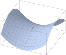 A saddle point
Consider, for purposes of illustration, a mountainous landscape M. If f is the function
 sending each point to its elevation, then the inverse image of a point in
  (a level set) is simply a contour line. Each connected component of a contour line is either a point, a simple closed curve, or a closed curve with a double point. Contour lines may also have points of higher order (triple points, etc.), but these are unstable and may be removed by a slight deformation of the landscape. Double points in contour lines occur at saddle points, or passes. Saddle points are points where the surrounding landscape curves up in one direction and down in the other.
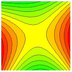
 Contour lines around a saddle point
Imagine flooding this landscape with water. Then, assuming the ground is porous, the region covered by water when the water reaches an elevation of a is f−1 (-∞, a], or the points with elevation less than or equal to a. Consider how the topology of this region changes as the water rises. It appears, intuitively, that it does not change except when a passes the height of a critical point; that is, a point where the gradient of f is 0. In other words, it does not change except when the water either (1) starts filling a basin, (2) covers a saddle (a mountain pass), or (3) submerges a peak.
 The torus
To each of these three types of critical points - basins, passes, and peaks (also called minima, saddles, and maxima) - one associates a number called the index. Intuitively speaking, the index of a critical point b is the number of independent directions around b in which f decreases. Therefore, the indices of basins, passes, and peaks are 0, 1, and 2, respectively.
Define Ma as f−1(-∞, a]. Leaving the context of topography, one can make a similar analysis of how the topology of Ma changes as a increases when M is a torus oriented as in the image and f is projection on a vertical axis, taking a point to its height above the plane.
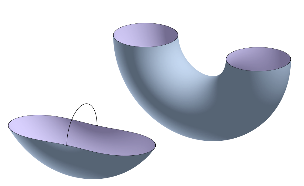
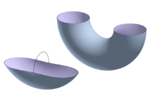 These figures are homotopy equivalent
 These figures are homotopy equivalent
Starting from the bottom of the torus, let p, q, r, and s be the four critical points of index 0, 1, 1, and 2, respectively. When a is less than 0, Ma is the empty set. After a passes the level of p, when 0<a<f(q), then Ma is a disk, which is homotopy equivalent to a point (a 0-cell), which has been "attached" to the empty set. Next, when a exceeds the level of q, and f(q)<a<f(r), then Ma is a cylinder, and is homotopy equivalent to a disk with a 1-cell attached (image at left). Once a passes the level of r, and f(r)<a<f(s), then Ma is a torus with a disk removed, which is homotopy equivalent to a cylinder with a 1-cell attached (image at right). Finally, when a is greater than the critical level of s, Ma is a torus. A torus, of course, is the same as a torus with a disk removed with a disk (a 2-cell) attached.
We therefore appear to have the following rule: the topology of Mα does not change except when α passes the height of a critical point, and when α passes the height of a critical point of index γ, a γ-cell is attached to Mα. This does not address the question of what happens when two critical points are at the same height. That situation can be resolved by a slight perturbation of f. In the case of a landscape (or a manifold embedded in Euclidean space), this perturbation might simply be tilting the landscape slightly, or rotating the coordinate system.
This rule, however, is false as stated. To see this, let M equal R and let f(x)=x3. Then 0 is a critical point of f, but the topology of Mα does not change when α passes 0. In fact, the concept of index does not make sense. The problem is that the second derivative is also 0 at 0. This kind of situation is called a degenerate critical point. Note that this situation is unstable: by rotating the coordinate system under the graph, the degenerate critical point either is removed or breaks up into two non-degenerate critical points.
Formal development
For a real-valued smooth function f : M → R on a differentiable manifold M, the points where the differential of f vanishes are called critical points of f and their images under f are called critical values. If at a critical point b, the matrix of second partial derivatives (the Hessian matrix) is non-singular, then b is called a non-degenerate critical point; if the Hessian is singular then b is a degenerate critical point.
For the functions
from R to R, f has a critical point at the origin if b=0, which is non-degenerate if c≠0 (i.e. f is of the form a+cx2+...) and degenerate if c=0 (i.e. f is of the form a+dx3+...). A less trivial example of a degenerate critical point is the origin of the monkey saddle.
The index of a non-degenerate critical point b of f is the dimension of the largest subspace of the tangent space to M at b on which the Hessian is negative definite. This corresponds to the intuitive notion that the index is the number of directions in which f decreases. The degeneracy and index of a critical point are independent of the choice the local coordinate system used, as shown by Sylvester's Law.
The Morse lemma
Let b be a non-degenerate critical point of f : M → R. Then there exists a chart (x1, x2, ..., xn) in a neighborhood U of b such that xi(b) = 0 for all i and
throughout U. Here α is equal to the index of f at b. As a corollary of the Morse lemma we see that non-degenerate critical points are isolated. (For a generalization, see Morse-Palais lemma).
For functions from R2 to R with a critical point at the origin, the Morse lemma implies that after rotation of coordinates f will be of the form
which will be degenerate if A = 0 or B = 0.
A smooth real-valued function on a manifold M is a Morse function if it has no degenerate critical points. A basic result of Morse theory says that almost all functions are Morse functions. Technically, the Morse functions form an open, dense subset of all smooth functions M → R in the C2 topology. This is sometimes expressed as "a typical function is Morse." or "a generic function is Morse".
As indicated before, we are interested in the question of when the topology of Ma = f−1(-∞, a] changes as a varies. Half of the answer to this question is given by the following theorem.
- Theorem. Suppose f is a smooth real-valued function on M, a < b, f−1[a, b] is compact, and there are no critical values between a and b. Then Ma is diffeomorphic to Mb, and Mb deformation retracts onto Ma.
It is also of interest to know how the topology of Ma changes when a passes a critical point. The following theorem answers that question.
- Theorem. Suppose f is a smooth real-valued function on M and p is a non-degenerate critical point of f of index γ, and that f(p) = q. Suppose f−1[q − ε, q + ε] is compact and contains no critical points besides p. Then Mq + ε is homotopy equivalent to Mq − ε with a γ-cell attached.
These results generalize and formalize the 'rule' stated in the previous section. As was mentioned, the rule as stated is incorrect; these theorems correct it.
Using the two previous results and the fact that there exists a Morse function on any differentiable manifold, one can prove that any differentiable manifold is a CW complex with an n-cell for each critical point of index n. To do this, one needs the technical fact that one can arrange to have a single critical point on each critical level, which is usually proven by using gradient-like vector fields to rearrange the critical points.
The Morse inequalities
Morse theory can be used to prove some strong results on the homology of manifolds. The number of critical points of index γ of f: M → R is equal to the number of γ cells in the CW structure on M obtained from "climbing" f. Using the fact that the alternating sum of the ranks of the homology groups of a topological space is equal to the alternating sum of the ranks of the chain groups from which the homology is computed, then by using the cellular chain groups (see cellular homology) it is clear that the Euler characteristic χ(M) is equal to the sum
where Cγ is the number of critical points of index γ. Also by cellular homology, the rank of the nth homology group of a CW complex M is less than or equal to the number of n-cells in M. Therefore the rank of the γth homology group,i.e., the Betti number bγ(M), is less than or equal to the number of critical points of index γ of a Morse function on M. These facts can be strengthened to obtain the Morse inequalities:
In particular, for any
we have
This gives a powerful tool to study manifold topology. Suppose on a closed manifold there exists a Morse function
 with precisely k critical points. In what way does the existence of the function f restricts M? The case k = 2 was studied by Reeb in 1952; Reeb sphere theorem states that M is homeomorphic to a sphere Sn. The case k = 3 is possible only in a small number of low dimensions, and M is homeomorphic to an Eells–Kuiper manifold.
Morse homology
Morse homology is a particularly easy way to understand approach to the homology of smooth manifolds. It is defined using a generic choice of Morse function and Riemannian metric. The basic theorem is that the resulting homology is an invariant of the manifold (i.e. independent of the function and metric) and isomorphic to the singular homology of the manifold; this implies that the Morse and singular Betti numbers agree and gives an immediate proof of the Morse inequalities. An infinite dimensional analog of Morse homology is known as Floer homology.
Ed Witten developed another related approach to Morse theory in 1982 using harmonic functions.
Morse–Bott theory
The notion of a Morse function can be generalized to consider functions that have nondegenerate manifolds of critical points.
Definition
A Morse–Bott function is a smooth function on a manifold whose critical set is a closed submanifold and whose Hessian is non-degenerate in the normal direction. (Equivalently, the kernel of the Hessian at a critical point equals the tangent space to the critical submanifold.) A Morse function is the special case where the critical manifolds are zero-dimensional (so the Hessian at critical points is non-degenerate in every direction, i.e., has no kernel).
The index is most naturally thought of as a pair
where i− is the dimension of the unstable manifold at a given point of the critical manifold, and i+ is i− plus the dimension of the critical manifold. If the Morse-Bott function is perturbed by a small function on the critical locus, the index of all critical points of the perturbed function on a critical manifold of the unperturbed function will lie between i− and i+).
Morse-Bott functions are useful because generic Morse functions are difficult to work with; the functions one can visualize, and with which one can easily calculate, typically have symmetries. They often lead to positive-dimensional critical manifolds. Raoul Bott used Morse-Bott theory in his original proof of the Bott periodicity theorem.
Round functions are examples of Morse-Bott functions, where the critical sets are (disjoint unions of) circles.
Morse homology can also be formulated for Morse-Bott functions; the differential in Morse-Bott homology is computed by a spectral sequence. Frederic Bourgeois developed a neat approach in the course of his work on a Morse-Bott version of symplectic field theory.
See also
- Discrete Morse theory
- Digital Morse theory
- Lusternik–Schnirelmann category
- Lagrangian Grassmannian
- Morse–Smale system
- Sard's lemma
- Stratified Morse theory
References
- Bott, Raoul (1988). Morse Theory Indomitable. Publications Mathématiques de l'IHÉS. 68, 99–114.
- Bott, Raoul (1982). Lectures on Morse theory, old and new., Bull. Amer. Math. Soc. (N.S.) 7, no. 2, 331–358.
- Cayley, Arthur (1859). On Contour and Slope Line. The Philosophical Magazine 18 (120), 264-268.
- Guest, Martin (April 15, 2001). "Morse Theory in the 1990's". http://www.comp.metro-u.ac.jp/~martin/RESEARCH/mg.ps, survey article; arXiv abstract.
- Matsumoto, Yukio (2002). An Introduction to Morse Theory
- Maxwell, James Clerk (1870). On Hills and Dales. The Philosophical Magazine 40 (269), 421–427.
- Milnor, John (1963). Morse Theory. Princeton University Press. ISBN 0-691-08008-9. A classic advanced reference in mathematics and mathematical physics.
- Milnor, John (1965). Lectures on the h-Cobordism theorem - scans available here
- Morse, Marston (1934). "The Calculus of Variations in the Large", American Mathematical Society Colloquium Publication 18; New York.
- Matthias Schwarz: Morse Homology, Birkhäuser, 1993.
- Seifert, Herbert & Threlfall, William (1938). Variationsrechnung im Grossen
- Witten, Edward (1982). Supersymmetry and Morse theory. J. Differential Geom. 17 (1982), no. 4, 661–692.
Categories:- Morse theory
- Smooth functions
- Lemmas


Wikimedia Foundation. 2010.