Weierstrass's elliptic functions

In mathematics, Weierstrass's elliptic functions are elliptic functions that take a particularly simple form; they are named for Karl Weierstrass. This class of functions are also referred to as p-functions and generally written using the symbol ℘ (or $\wp$) (a stylised letter p called Weierstrass p).

Symbol for Weierstrass P function

Definitions

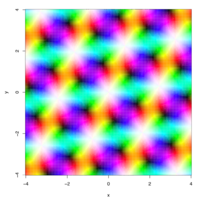
Weierstrass P function defined over a subset of the complex plane using a standard visualization technique in which white corresponds to a pole, black to a zero, and maximal saturation to $\left|f(z)\right|=\left|f(x+iy)\right|=1\;.$ Note the regular lattice of poles, and two interleaving lattices of zeros.

The Weierstrass elliptic function can be defined in three closely related ways, each of which possesses certain advantages. One is as a function of a complex variable z and a lattice Λ in the complex plane. Another is in terms of z and two complex numbers ω₁ and ω₂ defining a pair of generators, or periods, for the lattice. The third is in terms z and of a modulus τ in the upper half-plane. This is related to the previous definition by τ = ω₂/ω₁, which by the conventional choice on the pair of periods is in the upper half-plane. Using this approach, for fixed z the Weierstrass functions become modular functions of τ.

In terms of the two periods, Weierstrass's elliptic function is an elliptic function with periods ω₁ and ω₂ defined as

$\wp(z;\omega_1,\omega_2)=\frac{1}{z^2}+ \sum_{(m,n) \ne (0,0)} \left\{ \frac{1}{(z+m\omega_1+n\omega_2)^2}- \frac{1}{\left(m\omega_1+n\omega_2\right)^2} \right\}.$

Then $\Lambda=\{m\omega_1+n\omega_2:m,n\in\mathbb{Z}\}$ are the points of the period lattice, so that

$\wp(z;\Lambda)=\wp(z;\omega_1,\omega_2)$

for any pair of generators of the lattice defines the Weierstrass function as a function of a complex variable and a lattice.

If τ is a complex number in the upper half-plane, then

$\wp(z;\tau) = \wp(z;1,\tau) = \frac{1}{z^2} + \sum_{(m,n) \ne (0,0)}\left\{ {1 \over (z+m+n\tau)^2} - {1 \over (m+n\tau)^2}\right\}.$

The above sum is homogeneous of degree minus two, from which we may define the Weierstrass ℘ function for any pair of periods, as

$\wp(z;\omega_1,\omega_2) = \frac{\wp(\frac{z}{\omega_1}; \frac{\omega_2}{\omega_1})}{\omega_1^2}.$

We may compute ℘ very rapidly in terms of theta functions; because these converge so quickly, this is a more expeditious way of computing ℘ than the series we used to define it. The formula here is

$\wp(z; \tau) = \pi^2 \vartheta^2(0;\tau) \vartheta_{10}^2(0;\tau){\vartheta_{01}^2(z;\tau) \over \vartheta_{11}^2(z;\tau)}-{\pi^2 \over {3}}\left[\vartheta^4(0;\tau) + \vartheta_{10}^4(0;\tau)\right]$

There is a second-order pole at each point of the period lattice (including the origin). With these definitions, $\wp(z)$ is an even function and its derivative with respect to z, ℘′, an odd function.

Further development of the theory of elliptic functions shows that the condition on Weierstrass's function (correctly called pe) is determined up to addition of a constant and multiplication by a non-zero constant by the condition on the poles alone, amongst all meromorphic functions with the given period lattice.

Invariants

The real part of the invariant g₃ as a function of the nome q on the unit disk.

The imaginary part of the invariant g₃ as a function of the nome q on the unit disk.

If points close to the origin are considered the appropriate Laurent series is

$\wp(z;\omega_1,\omega_2)=z^{-2}+\frac{1}{20}g_2z^2+\frac{1}{28}g_3z^4+O(z^6)$

where

$g_2= 60\sum_{(m,n) \neq (0,0)} (m\omega_1+n\omega_2)^{-4} \quad \text{and} \quad g_3=140\sum_{(m,n) \neq (0,0)} (m\omega_1+n\omega_2)^{-6}.$

The numbers g₂ and g₃ are known as the invariants—they are two terms out of the Eisenstein series.

Note that g₂ and g₃ are homogeneous functions of degree −4 and −6; that is,

g₂(λω₁,λω₂) = λ ^{− 4}g₂(ω₁,ω₂)

and

g₃(λω₁,λω₂) = λ ^{− 6}g₃(ω₁,ω₂).

Thus, by convention, one frequently writes g₂ and g₃ in terms of the half-period ratio τ = ω₂ / ω₁ and take τ to lie in the upper half-plane. Thus, g₂(τ) = g₂(1,ω₂ / ω₁) and g₃(τ) = g₃(1,ω₂ / ω₁).

The Fourier series for g₂ and g₃ can be written in terms of the square of the nome q = exp(iπτ) as

$g_2(\tau)=\frac{4\pi^4}{3} \left[ 1+ 240\sum_{k=1}^\infty \sigma_3(k) q^{2k} \right]$

and

$g_3(\tau)=\frac{8\pi^6}{27} \left[ 1- 504\sum_{k=1}^\infty \sigma_5(k) q^{2k} \right]$

where σ_a(k) is the divisor function. This formula may be rewritten in terms of Lambert series.

The invariants may be expressed in terms of Jacobi's theta functions. This method is very convenient for numerical calculation: the theta functions converge very quickly. In the notation of Abramowitz and Stegun, but denoting the primitive half-periods by ω₁,ω₂, the invariants satisfy

$g_2(\omega_1,\omega_2)= \frac{\pi^4}{12\omega_1^4} \left( \theta_2(0,q)^8-\theta_3(0,q)^4\theta_2(0,q)^4+\theta_3(0,q)^8 \right)$

and

$g_3(\omega_1,\omega_2)= \frac{\pi^6}{(2\omega_1)^6} \left[ \frac{8}{27}\left(\theta_2(0,q)^{12}+\theta_3(0,q)^{12}\right)\right.$

$\left. {} - \frac{4}{9}\left(\theta_2(0,q)^4+\theta_3(0,q)^4\right)\cdot \theta_2(0,q)^4\theta_3(0,q)^4 \right]$

where τ = ω₂ / ω₁ is the half-period ratio and q = e^πiτ is the nome.

Special cases

If the invariants are g₂ = 0, g₃ = 1, then this is known as the equianharmonic case; g₂ = 1, g₃ = 0 is the lemniscatic case.

Differential equation

With this notation, the ℘ function satisfies the following differential equation:

$[\wp'(z)]^2 = 4[\wp(z)]^3-g_2\wp(z)-g_3, \,$

where dependence on ω₁ and ω₂ is suppressed.

This relation can be quickly verified by comparing the poles of both sides, for example, the pole at z = 0 of lhs is

$[\wp'(z)]^2|_{z=0}\sim \frac{4}{z^6}-\frac{24}{z^2}\sum \frac{1}{(m\omega_1+n\omega_2)^4}-80\sum \frac{1}{(m\omega_1+n\omega_2)^6}$

while the pole at z = 0 of

$[\wp(z)]^3|_{z=0}\sim \frac{1}{z^6}+\frac{9}{z^2}\sum \frac{1}{(m\omega_1+n\omega_2)^4}+15\sum \frac{1}{(m\omega_1+n\omega_2)^6}.$

Comparing these two yields the relation above.

Integral equation

The Weierstrass elliptic function can be given as the inverse of an elliptic integral. Let

$u = \int_y^\infty \frac {ds} {\sqrt{4s^3 - g_2s -g_3}}.$

Here, g₂ and g₃ are taken as constants. Then one has

$y=\wp(u).$

The above follows directly by integrating the differential equation.

Modular discriminant

The real part of the discriminant as a function of the nome q on the unit disk.

The modular discriminant Δ is defined as

$\Delta=g_2^3-27g_3^2. \,$

This is studied in its own right, as a cusp form, in modular form theory (that is, as a function of the period lattice).

Note that Δ = (2π)¹²η²⁴ where η is the Dedekind eta function.

The presence of 24 can be understood by connection with other occurrences, as in the eta function and the Leech lattice.

The discriminant is a modular form of weight 12. That is, under the action of the modular group, it transforms as

$\Delta \left( \frac {a\tau+b} {c\tau+d}\right) = \left(c\tau+d\right)^{12} \Delta(\tau)$

with τ being the half-period ratio, and a,b,c and d being integers, with ad − bc = 1.

The constants e₁, e₂ and e₃

Consider the cubic polynomial equation 4t³ − g₂t − g₃ = 0 with roots e₁, e₂, and e₃. If the discriminant $\Delta = g_{2}^{3} - 27 g_{3}^{2}$ is not zero, no two of these roots are equal. Since the quadratic term of this cubic polynomial is zero, the roots are related by the equation

$e_1+e_2+e_3=0. \,$

The linear and constant coefficients (g₂ and g₃, respectively) are related to the roots by the equations^[1]

$g_2 = -4 \left( e_1 e_2 + e_1 e_3 + e_2 e_3 \right) = 2 \left( e_1^2 + e_2^2 + e_3^2 \right) \,$

$g_3 = 4 e_1 e_2 e_3. \,$

In the case of real invariants, the sign of Δ determines the nature of the roots. If Δ > 0, all three are real and it is conventional to name them so that e₁ > e₂ > e₃. If Δ < 0, it is conventional to write e₁ = − α + βi (where $\alpha\geq 0$, β > 0), whence $e_3=\overline{e_1}$ and e₂ is real and non-negative.

The half-periods ω₁ and ω₂ of Weierstrass' elliptic function are related to the roots

$\wp(\omega_1)=e_1\qquad \wp(\omega_2)=e_2\qquad \wp(\omega_3)=e_3$

where ω₃ = − (ω₁ + ω₂). Since the derivative of Weierstrass' elliptic function equals the above cubic polynomial of the function's value, $\wp'(\omega_i)=0$ for i = 1,2,3; if the function's value equals a root of the polynomial, the derivative is zero.

If g₂ and g₃ are real and Δ > 0, the e_i are all real, and $\wp()$ is real on the perimeter of the rectangle with corners 0, ω₃, ω₁ + ω₃, and ω₁. If the roots are ordered as above (e₁ > e₂ > e₃), then the first half-period is completely real

$\omega_{1} = \int_{e_{1}}^{\infty} \frac{dz}{\sqrt{4z^{3} - g_{2}z - g_{3}}}$

whereas the third half-period is completely imaginary

$\omega_{3} = i \int_{-e_{3}}^{\infty} \frac{dz}{\sqrt{4z^{3} - g_{2}z - g_{3}}}.$

Addition theorems

The Weierstrass elliptic functions have several properties that may be proved:

$\det\begin{bmatrix} \wp(z) & \wp'(z) & 1\\ \wp(y) & \wp'(y) & 1\\ \wp(z+y) & -\wp'(z+y) & 1 \end{bmatrix}=0$

(a symmetrical version would be

$\det\begin{bmatrix} \wp(u) & \wp'(u) & 1\\ \wp(v) & \wp'(v) & 1\\ \wp(w) & \wp'(w) & 1 \end{bmatrix}=0$

where u + v + w = 0).

Also

$\wp(z+y)=\frac{1}{4} \left\{ \frac{\wp'(z)-\wp'(y)}{\wp(z)-\wp(y)} \right\}^2 -\wp(z)-\wp(y).$

and the duplication formula

$\wp(2z)= \frac{1}{4}\left\{ \frac{\wp''(z)}{\wp'(z)}\right\}^2-2\wp(z),$

unless 2z is a period.

The case with 1 a basic half-period

If ω₁ = 1, much of the above theory becomes simpler; it is then conventional to write τ for ω₂. For a fixed τ in the upper half-plane, so that the imaginary part of τ is positive, we define the Weierstrass ℘ function by

$\wp(z;\tau) =\frac{1}{z^2} + \sum_{(m,n) \ne (0,0)}{1 \over (z+m+n\tau)^2} - {1 \over (m+n\tau)^2}.$

The sum extends over the lattice {n+mτ : n and m in Z} with the origin omitted. Here we regard τ as fixed and ℘ as a function of z; fixing z and letting τ vary leads into the area of elliptic modular functions.

General theory

℘ is a meromorphic function in the complex plane with a double pole at each lattice points. It is doubly periodic with periods 1 and τ; this means that ℘ satisfies

$\wp(z+1) = \wp(z+\tau) = \wp(z).$

The above sum is homogeneous of degree minus two, and if c is any non-zero complex number,

$\wp(cz;c\tau) = \wp(z;\tau)/c^2$

from which we may define the Weierstrass ℘ function for any pair of periods. We also may take the derivative (of course, with respect to z) and obtain a function algebraically related to ℘ by

$\wp'^2 = 4\wp^3 - g_2 \wp - g_3$

where g₂ and g₃ depend only on τ, being modular forms. The equation

Y² = 4X³ − g₂X − g₃

defines an elliptic curve, and we see that $(\wp, \wp')$ is a parametrization of that curve.

The totality of meromorphic doubly periodic functions with given periods defines an algebraic function field, associated to that curve. It can be shown that this field is

$\Bbb{C}(\wp, \wp'),$

so that all such functions are rational functions in the Weierstrass function and its derivative.

We can also wrap a single period parallelogram into a torus, or donut-shaped Riemann surface, and regard the elliptic functions associated to a given pair of periods to be functions defined on that Riemann surface.

The roots e₁, e₂, and e₃ of the equation 4X³ − g₂X − g₃ depend on τ and can be expressed in terms of theta functions; we have

$e_1(\tau) = \tfrac{1}{3} \pi^2(\vartheta^4(0;\tau) + \vartheta_{01}^4(0;\tau)),$

$e_2(\tau) = -\tfrac{1}{3} \pi^2(\vartheta^4(0;\tau) + \vartheta_{10}^4(0;\tau)),$

$e_3(\tau) = \tfrac{1}{3} \pi^2(\vartheta_{10}^4(0;\tau) - \vartheta_{01}^4(0;\tau)).$

Since g₂ = − 4(e₁e₂ + e₂e₃ + e₃e₁) and g₃ = 4e₁e₂e₃ we have these in terms of theta functions also.

We may also express ℘ in terms of theta functions; because these converge very rapidly, this is a more expeditious way of computing ℘ than the series we used to define it.

$\wp(z; \tau) = \pi^2 \vartheta^2(0;\tau) \vartheta_{10}^2(0;\tau){\vartheta_{01}^2(z;\tau) \over \vartheta_{11}^2(z;\tau)} + e_2(\tau).$

The function ℘ has two zeros (modulo periods) and the function ℘′ has three. The zeros of ℘′ are easy to find: since ℘′ is an odd function they must be at the half-period points. On the other hand it is very difficult to express the zeros of ℘ by closed formula, except for special values of the modulus (e.g. when the period lattice is the Gaussian integers). An expression was found, by Zagier and Eichler.^[2]

The Weierstrass theory also includes the Weierstrass zeta function, which is an indefinite integral of ℘ and not doubly periodic, and a theta function called the Weierstrass sigma function, of which his zeta-function is the log-derivative. The sigma-function has zeros at all the period points (only), and can be expressed in terms of Jacobi's functions. This gives one way to convert between Weierstrass and Jacobi notations.

The Weierstrass sigma-function is an entire function; it played the role of 'typical' function in a theory of random entire functions of J. E. Littlewood.

Relation to Jacobi elliptic functions

For numerical work, it is often convenient to calculate the Weierstrass elliptic function in terms of the Jacobi's elliptic functions. The basic relations are^[3]

$\wp(z) = e_{3} + \frac{e_{1} - e_{3}}{\mathrm{sn}^{2}\,w} = e_{2} + \left( e_{1} - e_{3} \right) \frac{\mathrm{dn}^{2}\,w}{\mathrm{sn}^{2}\,w} = e_{1} + \left( e_{1} - e_{3} \right) \frac{\mathrm{cn}^{2}\,w}{\mathrm{sn}^{2}\,w}$

where e_1-3 are the three roots described above and where the modulus k of the Jacobi functions equals

$k \equiv \sqrt{\frac{e_{2} - e_{3}}{e_{1} - e_{3}}}$

and their argument w equals

$w \equiv z \sqrt{e_{1} - e_{3}}.$

Notes

1. ^ Abramowitz and Stegun, p. 629
2. ^ M. Eichler and D. Zagier, On the zeros of the Weierstrass ℘-Function, Mathematische Annalen, Volume 258, Number 4, December 1982.
3. ^ Korn GA, Korn TM (1961). Mathematical Handbook for Scientists and Engineers. New York: McGraw-Hill. pp. p. 721. LCCN 59-14456. 

References

• Abramowitz, Milton; Stegun, Irene A., eds. (1965), "Chapter 18", Handbook of Mathematical Functions with Formulas, Graphs, and Mathematical Tables, New York: Dover, pp. 627, ISBN 978-0486612720, MR0167642, http://www.math.sfu.ca/~cbm/aands/page_627.htm .
• N. I. Akhiezer, Elements of the Theory of Elliptic Functions, (1970) Moscow, translated into English as AMS Translations of Mathematical Monographs Volume 79 (1990) AMS, Rhode Island ISBN 0-8218-4532-2
• Tom M. Apostol, Modular Functions and Dirichlet Series in Number Theory, Second Edition (1990), Springer, New York ISBN 0-387-97127-0 (See chapter 1.)
• K. Chandrasekharan, Elliptic functions (1980), Springer-Verlag ISBN 0-387-15295-4
• Konrad Knopp, Funktionentheorie II (1947), Dover; Republished in English translation as Theory of Functions (1996), Dover ISBN 0-486-69219-1
• Serge Lang, Elliptic Functions (1973), Addison-Wesley, ISBN 0-201-04162-6
• Reinhardt, William P.; Walker, Peter L. (2010), "Weierstrass Elliptic and Modular Functions", in Olver, Frank W. J.; Lozier, Daniel M.; Boisvert, Ronald F. et al., NIST Handbook of Mathematical Functions, Cambridge University Press, ISBN 978-0521192255, MR2723248, http://dlmf.nist.gov/23 
• E. T. Whittaker and G. N. Watson, A course of modern analysis, Cambridge University Press, 1952, chapters 20 and 21

External links

• Weierstrass's elliptic functions on Mathworld.
• Elliptic functions, Hans Lundmark's Complex analysis page.