- Complex number
-
 A complex number can be visually represented as a pair of numbers forming a vector on a diagram called an Argand diagram, representing the complex plane. Re is the real axis, Im is the imaginary axis, and i is the square root of –1.
A complex number is a number consisting of a real part and an imaginary part. Complex numbers extend the idea of the one-dimensional number line to the two-dimensional complex plane by using the number line for the real part and adding a vertical axis to plot the imaginary part. In this way the complex numbers contain the ordinary real numbers while extending them in order to solve problems that would be impossible with only real numbers.
Complex numbers are used in many scientific fields, including engineering, electromagnetism, quantum physics, applied mathematics, and chaos theory. Italian mathematician Gerolamo Cardano is the first known to have introduced complex numbers; he called them "fictitious", during his attempts to find solutions to cubic equations in the 16th century.[1]
Contents
Introduction and definition
Complex numbers have been introduced to allow for solutions of certain equations that have no real solution: the equation
has no real solution x, since the square of x is 0 or positive, so x2 + 1 cannot be zero. Complex numbers are a solution to this problem. The idea is to enhance the real numbers by introducing a non-real number i whose square is −1, so that x = i and x = −i are the two solutions to the preceding equation.
Definition
A complex number is an expression of the form
where a and b are real numbers and i is the imaginary unit, satisfying i2 = −1. For example, −3.5 + 2i is a complex number.
The real number a of the complex number z = a + bi is called the real part of z and the real number b is the imaginary part.[2] They are denoted Re(z) or ℜ(z) and Im(z) or ℑ(z), respectively. For example,
Some authors write a+ib instead of a+bi. In some disciplines (in particular, electrical engineering, where i is a symbol for current), in order to avoid notational conflict, the imaginary unit i is instead written as j, so complex numbers are written as a + bj or a + jb.
A real number a can usually be regarded as a complex number with an imaginary part of zero, that is to say, a + 0i. However the sets are defined differently and have slightly different operations defined, for instance comparison operations are not defined for complex numbers. Complex numbers whose real part is zero, that is to say, those of the form 0 + bi, are called imaginary numbers. It is common to write a for a + 0i and bi for 0 + bi. Moreover, when b is negative, it is common to write a − bi instead of a + (−b)i, for example 3 − 4i instead of 3 + (−4)i.
The set of all complex numbers is denoted by C or
 .
.The complex plane
Main article: Complex plane Figure 1: A complex number plotted as a point (red) and position vector (blue) on an Argand diagram; a + bi is the rectangular expression of the point.
A complex number can be viewed as a point or position vector in a two-dimensional Cartesian coordinate system called the complex plane or Argand diagram (see Pedoe 1988 and Solomentsev 2001), named after Jean-Robert Argand. The numbers are conventionally plotted using the real part as the horizontal component, and imaginary part as vertical (see Figure 1). These two values used to identify a given complex number are therefore called its Cartesian, rectangular, or algebraic form.
The defining characteristic of a position vector is that it has magnitude and direction. These are emphasised in a complex number's polar form and it turns out notably that the operations of addition and multiplication take on a very natural geometric character when complex numbers are viewed as position vectors: addition corresponds to vector addition while multiplication corresponds to multiplying their magnitudes and adding their arguments (i.e. the angles they make with the x axis). Viewed in this way the multiplication of a complex number by i corresponds to rotating a complex number counterclockwise through 90° about the origin: (a + bi)i = ai + bi2 = − b + ai.
History in brief
- Main section: History
The solution of a general cubic equation in radicals (without trigonometric functions) may require intermediate calculations containing the square roots of negative numbers, even when the final solutions are real numbers, a situation known as casus irreducibilis. This conundrum led Italian mathematician Gerolamo Cardano to conceive of complex numbers in around 1545, though his understanding was rudimentary.
Work on the problem of general polynomials ultimately led to the fundamental theorem of algebra, which shows that with complex numbers, a solution exists to every polynomial equation of degree one or higher. Complex numbers thus form an algebraically closed field, where any polynomial equation has a root.
Many mathematicians contributed to the full development of complex numbers. The rules for addition, subtraction, multiplication, and division of complex numbers were developed by the Italian mathematician Rafael Bombelli.[3] A more abstract formalism for the complex numbers was further developed by the Irish mathematician William Rowan Hamilton, who extended this abstraction to the theory of quaternions.
Elementary operations
Conjugation
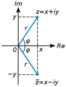 Geometric representation of z and its conjugate
 in the complex plane
The complex conjugate of the complex number z = x + yi is defined to be x − yi. It is denoted
or  . Geometrically, is the "reflection" of z about the real axis. In particular, conjugating twice gives the original complex number:
  .
.The real and imaginary parts of a complex number can be extracted using the conjugate:
Moreover, a complex number is real if and only if it equals its conjugate.
Conjugation distributes over the standard arithmetic operations:
The reciprocal of a nonzero complex number z = x + yi is given by
This formula can be used to compute the multiplicative inverse of a complex number if it is given in rectangular coordinates. Inversive geometry, a branch of geometry studying more general reflections than ones about a line, can also be expressed in terms of complex numbers.
Addition and subtraction
 Addition of two complex numbers can be done geometrically by constructing a parallelogram.
Complex numbers are added by adding the real and imaginary parts of the summands. That is to say:
Similarly, subtraction is defined by
Using the visualization of complex numbers in the complex plane, the addition has the following geometric interpretation: the sum of two complex numbers A and B, interpreted as points of the complex plane, is the point X obtained by building a parallelogram three of whose vertices are 0, A and B. Equivalently, X is the point such that the triangles with vertices 0, A, B, and X, B, A, are congruent.
Multiplication and division
The multiplication of two complex numbers is defined by the following formula:
In particular, the square of the imaginary unit is −1:
The preceding definition of multiplication of general complex numbers is the natural way of extending this fundamental property of the imaginary unit. Indeed, treating i as a variable, the formula follows from this
 (distributive law)
-
 (commutative law of addition—the order of the summands can be changed)
 (commutative law of multiplication—the order of the factors can be changed)
 (fundamental property of the imaginary unit).
-
The division of two complex numbers is defined in terms of complex multiplication, which is described above, and real division:
Division can be defined in this way because of the following observation:
As shown earlier, c − di is the complex conjugate of the denominator c + di. The real part c and the imaginary part d of the denominator must not both be zero for division to be defined.
Square root
The square roots of a + bi (with b ≠ 0) are
 , where
and
where sgn is the signum function. This can be seen by squaring
to obtain a + bi.[4][5] Here  is called the modulus of a + bi, and the square root with non-negative real part is called the principal square root.
Polar form
Main article: Polar coordinate system Figure 2: The argument φ and modulus r locate a point on an Argand diagram; r(cos ϕ + isin ϕ) or reiϕ are polar expressions of the point.
Absolute value and argument
Another way of encoding points in the complex plane other than using the x- and y-coordinates is to use the distance of a point P to O, the point whose coordinates are (0, 0) (origin), and the angle of the line through P and O. This idea leads to the polar form of complex numbers.
The absolute value (or modulus or magnitude) of a complex number z = x + yi is
If z is a real number (i.e., y = 0), then r = |x|. In general, by Pythagoras' theorem, r is the distance of the point P representing the complex number z to the origin.
The argument or phase of z is the angle of the radius OP with the positive real axis, and is written as arg(z). As with the modulus, the argument can be found from the rectangular form x + iy:[6]
The value of φ must always be expressed in radians. It can change by any multiple of 2π and still give the same angle. Hence, the arg function is sometimes considered as multivalued. Normally, as given above, the principal value in the interval ( − π,π] is chosen. Values in the range [0,2π) are obtained by adding 2π if the value is negative. The polar angle for the complex number 0 is undefined, but arbitrary choice of the angle 0 is common.
The value of φ equals the result of atan2: φ = atan2(imaginary,real).
Together, r and φ give another way of representing complex numbers, the polar form, as the combination of modulus and argument fully specify the position of a point on the plane. Recovering the original rectangular co-ordinates from the polar form is done by the formula called trigonometric form
Using Euler's formula this can be written as
Using the cis function, this is sometimes abbreviated to
In angle notation, often used in electronics to represent a phasor with amplitude r and phase φ it is written as[7]
Multiplication, division and exponentiation in polar form
 Multiplication of 2+i (blue triangle) and 3+i (red triangle). The red triangle is rotated to match the vertex of the blue one and stretched by √5, the length of the hypotenuse of the blue triangle.
The relevance of representing complex numbers in polar form stems from the fact that the formulas for multiplication, division and exponentiation are simpler than the ones using Cartesian coordinates. Given two complex numbers z1 = r1(cos φ1 + isin φ1) and z2 =r2(cos φ2 + isin φ2) the formula for multiplication is
In other words, the absolute values are multiplied and the arguments are added to yield the polar form of the product. For example, multiplying by i corresponds to a quarter-rotation counter-clockwise, which gives back i 2 = −1. The picture at the right illustrates the multiplication of
Since the real and imaginary part of 5+5i are equal, the argument of that number is 45 degrees, or π/4 (in radian). On the other hand, it is also the sum of the angles at the origin of the red and blue triangle are arctan(1/3) and arctan(1/2), respectively. Thus, the formula
holds. As the arctan function can be approximated highly efficiently, formulas like this—known as Machin-like formulas—are used for high-precision approximations of π.
Similarly, division is given by
This also implies de Moivre's formula for exponentiation of complex numbers with integer exponents:
The n-th roots of z are given by
for any integer k satisfying 0 ≤ k ≤ n − 1. Here
![\sqrt[n]{r}](1/0c1dda2d990c60ca5ef80cd446e594db.png) is the usual (positive) nth root of the positive real number r. While the nth root of a positive real number r is chosen to be the positive real number c satisfying cn = x there is no natural way of distinguishing one particular complex nth root of a complex number. Therefore, the nth root of z is considered as a multivalued function (in z), as opposed to a usual function f, for which f(z) is a uniquely defined number. Formulas such as
is the usual (positive) nth root of the positive real number r. While the nth root of a positive real number r is chosen to be the positive real number c satisfying cn = x there is no natural way of distinguishing one particular complex nth root of a complex number. Therefore, the nth root of z is considered as a multivalued function (in z), as opposed to a usual function f, for which f(z) is a uniquely defined number. Formulas such as(which holds for positive real numbers), do in general not hold for complex numbers.
Properties
Field structure
The set C of complex numbers is a field. Briefly, this means that the following facts hold: first, any two complex numbers can be added and multiplied to yield another complex number. Second, for any complex number a, its negative −a is also a complex number; and third, every nonzero complex number has a reciprocal complex number. Moreover, these operations satisfy a number of laws, for example the law of commutativity of addition and multiplication for any two complex numbers z1 and z2:
These two laws and the other requirements on a field can be proven by the formulas given above, using the fact that the real numbers themselves form a field.
Unlike the reals, C is not an ordered field, that is to say, it is not possible to define a relation z1 < z2 that is compatible with the addition and multiplication. In fact, in any ordered field, the square of any element is necessarily positive, so i2 = −1 precludes the existence of an ordering on C.
When the underlying field for a mathematical topic or construct is the field of complex numbers, the thing's name is usually modified to reflect that fact. For example: complex analysis, complex matrix, complex polynomial, and complex Lie algebra.
Solutions of polynomial equations
Given any complex numbers (called coefficients) a0, ..., an, the equation
has at least one complex solution z, provided that at least one of the higher coefficients, a1, ..., an, is nonzero. This is the statement of the fundamental theorem of algebra. Because of this fact, C is called an algebraically closed field. This property does not hold for the field of rational numbers Q (the polynomial x2 − 2 does not have a rational root, since √2 is not a rational number) nor the real numbers R (the polynomial x2 + a does not have a real solution for a > 0, since the square of x is positive for any real number x).
There are various proofs of this theorem, either by analytic methods such as Liouville's theorem, or topological ones such as the winding number, or a proof combining Galois theory and the fact that any real polynomial of odd degree has at least one root.
Because of this fact, theorems that hold "for any algebraically closed field", apply to C. For example, any complex matrix has at least one (complex) eigenvalue.
Algebraic characterization
The field C has the following three properties: first, it has characteristic 0. This means that 1 + 1 + ... + 1 ≠ 0 for any number of summands (all of which equal one). Second, its transcendence degree over Q, the prime field of C is the cardinality of the continuum. Third, it is algebraically closed (see above). It can be shown that any field having these properties is isomorphic (as a field) to C. For example, the algebraic closure of Qp also satisfies these three properties, so these two fields are isomorphic. Also, C is isomorphic to the field of complex Puiseux series. However, specifying an isomorphism requires the axiom of choice. Another consequence of this algebraic characterization is that C contains many proper subfields which are isomorphic to C (the same is true of R, which contains many sub fields isomorphic to itself[citation needed]).
Characterization as a topological field
The preceding characterization of C describes the algebraic aspects of C, only. That is to say, the properties of nearness and continuity, which matter in areas such as analysis and topology, are not dealt with. The following description of C as a topological field (that is, a field that is equipped with a topology, which allows one to specify notions such as convergence) does take into account the topological properties. C contains a subset P (namely the set of positive real numbers) of nonzero elements satisfying the following three conditions:
- P is closed under addition, multiplication and taking inverses.
- If x and y are distinct elements of P, then either x − y or y − x is in P.
- If S is any nonempty subset of P, then S + P = x + P for some x in C.
Moreover, C has a nontrivial involutive automorphism
 (namely the complex conjugation), such that xx∗ is in P for any nonzero x in C.
Any field F with these properties can be endowed with a topology by taking the sets B(x, p) = {y | p − (y − x)(y − x)∗ ∈ P} as a base, where x ranges over the field and p ranges over P. With this topology F is isomorphic as a topological field to C.
The only connected locally compact topological fields are R and C. This gives another characterization of C as a topological field, since C can be distinguished from R because the nonzero complex numbers are connected, while the nonzero real numbers are not.
Formal construction
Formal development
Above, complex numbers have been defined by introducing i, the imaginary unit, as a symbol. More rigorously, the set C of complex numbers can be defined as the set R2 of ordered pairs (a, b) of real numbers. In this notation, the above formulas for addition and multiplication read
It is then just a matter of notation to express (a, b) as a + ib.
Though this low-level construction does accurately describe the structure of the complex numbers, the following equivalent definition reveals the algebraic nature of C more immediately. This characterization relies on the notion of fields and polynomials. A field is a set endowed with an addition, subtraction, multiplication and division operations which behave as is familiar from, say, rational numbers. For example, the distributive law
is required to hold for any three elements x, y and z of a field. The set R of real numbers does form a field. A polynomial p(X) with real coefficients is an expression of the form
where the a0, ..., an are real numbers. The usual addition and multiplication of polynomials endows the set R[X] of all such polynomials with a ring structure. This ring is called polynomial ring. The quotient ring R[X]/(X2+1) can be shown to be a field. This extension field contains two square roots of −1, namely (the cosets of) X and −X, respectively. (The cosets of) 1 and X form a basis of R[X]/(X2+1) as a real vector space, which means that each element of the extension field can be uniquely written as a linear combination in these two elements. Equivalently, elements of the extension field can be written as ordered pairs (a,b) of real numbers. Moreover, the above formulas for addition etc. correspond to the ones yielded by this abstract algebraic approach – the two definitions of the field C are said to be isomorphic (as fields). Together with the above-mentioned fact that C is algebraically closed, this also shows that C is an algebraic closure of R.
Matrix representation of complex numbers
Complex numbers can also be represented by 2×2 matrices that have the following form:
Here the entries a and b are real numbers. The sum and product of two such matrices is again of this form, and the sum and product of complex numbers corresponds to the sum and product of such matrices. The geometric description of the multiplication of complex numbers can also be phrased in terms of rotation matrices by using this correspondence between complex numbers and such matrices. Moreover, the square of the absolute value of a complex number expressed as a matrix is equal to the determinant of that matrix:
The conjugate
 corresponds to the transpose of the matrix.
Though this representation of complex numbers with matricies is the most common, many other representations arise from matrices other than
 that square to the negative of the identity matrix. See the article on 2 × 2 real matrices for other representations of complex numbers.
Complex analysis
 Color wheel graph of sin(1/z). Black parts inside refer to numbers having large absolute values.Main article: Complex analysis
The study of functions of a complex variable is known as complex analysis and has enormous practical use in applied mathematics as well as in other branches of mathematics. Often, the most natural proofs for statements in real analysis or even number theory employ techniques from complex analysis (see prime number theorem for an example). Unlike real functions which are commonly represented as two-dimensional graphs, complex functions have four-dimensional graphs and may usefully be illustrated by color coding a three-dimensional graph to suggest four dimensions, or by animating the complex function's dynamic transformation of the complex plane.
The notions of convergent series and continuous functions in (real) analysis have natural analogs in complex analysis. A sequence of complex numbers is said to converge if and only if its real and imaginary parts do. This is equivalent to the (ε, δ)-definition of limits, where the absolute value of real numbers is replaced by the one of complex numbers. From a more abstract point of view, C, endowed with the metric
is a complete metric space, which notably includes the triangle inequality
for any two complex numbers z1 and z2.
Like in real analysis, this notion of convergence is used to construct a number of elementary functions: the exponential function exp(z), also written ez, is defined as the infinite series
and the series defining the real trigonometric functions sine and cosine, as well as hyperbolic functions such as sinh also carry over to complex arguments without change. Euler's identity states:
for any real number φ, in particular
Unlike in the situation of real numbers, there is an infinitude of complex solutions z of the equation
for any complex number w ≠ 0. It can be shown that any such solution z—called complex logarithm of a—satisfies
where arg is the argument defined above, and ln the (real) natural logarithm. As arg is a multivalued function, unique only up to a multiple of 2π, log is also multivalued. The principal value of log is often taken by restricting the imaginary part to the interval (−π,π].
Complex exponentiation zω is defined as
Consequently, they are in general multi-valued. For ω = 1 / n, for some natural number n, this recovers the non-unicity of n-th roots mentioned above.
Holomorphic functions
A function f : C → C is called holomorphic if it satisfies the Cauchy-Riemann equations. For example, any R-linear map C → C can be written in the form
with complex coefficients a and b. This map is holomorphic if and only if b = 0. The second summand
 is real-differentiable, but does not satisfy the Cauchy-Riemann equations.
Complex analysis shows some features not apparent in real analysis. For example, any two holomorphic functions f and g that agree on an arbitrarily small open subset of C necessarily agree everywhere. Meromorphic functions, functions that can locally be written as f(z)/(z − z0)n with a holomorphic function f(z), still share some of the features of holomorphic functions. Other functions have essential singularities, such as sin(1/z) at z = 0.
Applications
Some applications of complex numbers are:
Control theory
In control theory, systems are often transformed from the time domain to the frequency domain using the Laplace transform. The system's poles and zeros are then analyzed in the complex plane. The root locus, Nyquist plot, and Nichols plot techniques all make use of the complex plane.
In the root locus method, it is especially important whether the poles and zeros are in the left or right half planes, i.e. have real part greater than or less than zero. If a system has poles that are
- in the right half plane, it will be unstable,
- all in the left half plane, it will be stable,
- on the imaginary axis, it will have marginal stability.
If a system has zeros in the right half plane, it is a nonminimum phase system.
Signal analysis
Complex numbers are used in signal analysis and other fields for a convenient description for periodically varying signals. For given real functions representing actual physical quantities, often in terms of sines and cosines, corresponding complex functions are considered of which the real parts are the original quantities. For a sine wave of a given frequency, the absolute value |z| of the corresponding z is the amplitude and the argument arg(z) the phase.
If Fourier analysis is employed to write a given real-valued signal as a sum of periodic functions, these periodic functions are often written as complex valued functions of the form
where ω represents the angular frequency and the complex number z encodes the phase and amplitude as explained above.
In electrical engineering, the Fourier transform is used to analyze varying voltages and currents. The treatment of resistors, capacitors, and inductors can then be unified by introducing imaginary, frequency-dependent resistances for the latter two and combining all three in a single complex number called the impedance. This approach is called phasor calculus. This use is also extended into digital signal processing and digital image processing, which utilize digital versions of Fourier analysis (and wavelet analysis) to transmit, compress, restore, and otherwise process digital audio signals, still images, and video signals.
Improper integrals
In applied fields, complex numbers are often used to compute certain real-valued improper integrals, by means of complex-valued functions. Several methods exist to do this; see methods of contour integration.
Quantum mechanics
The complex number field is relevant in the mathematical formulations of quantum mechanics, where complex Hilbert spaces provide the context for one such formulation that is convenient and perhaps most standard. The original foundation formulas of quantum mechanics – the Schrödinger equation and Heisenberg's matrix mechanics – make use of complex numbers.
Relativity
In special and general relativity, some formulas for the metric on spacetime become simpler if one takes the time variable to be imaginary. (This is no longer standard in classical relativity, but is used in an essential way in quantum field theory.) Complex numbers are essential to spinors, which are a generalization of the tensors used in relativity.
Dynamic equations
In differential equations, it is common to first find all complex roots r of the characteristic equation of a linear differential equation or equation system and then attempt to solve the system in terms of base functions of the form f(t) = ert. Likewise, in difference equations, the complex roots r of the characteristic equation of the difference equation system are used, to attempt to solve the system in terms of base functions of the form f(t) = r t.
Fluid dynamics
In fluid dynamics, complex functions are used to describe potential flow in two dimensions.
Fractals
Certain fractals are plotted in the complex plane, e.g. the Mandelbrot set and Julia sets.
Algebraic number theory
 Construction of a regular polygon using straightedge and compass.
As mentioned above, any nonconstant polynomial equation (in complex coefficients) has a solution in C. A fortiori, the same is true if the equation has rational coefficients. The roots of such equations are called algebraic numbers – they are a principal object of study in algebraic number theory. Compared to Q, the algebraic closure of Q, which also contains all algebraic numbers, C has the advantage of being easily understandable in geometric terms. In this way, algebraic methods can be used to study geometric questions and vice versa. With algebraic methods, more specifically applying the machinery of field theory to the number field containing roots of unity, it can be shown that it is not possible to construct a regular nonagon using only compass and straightedge – a purely geometric problem.
Another example are Pythagorean triples (a, b, c), that is to say integers satisfying
(which implies that the triangle having sidelengths a, b, and c is a right triangle). They can be studied by considering Gaussian integers, that is, numbers of the form x + iy, where x and y are integers.
Analytic number theory
Analytic number theory studies numbers, often integers or rationals, by taking advantage of the fact that they can be regarded as complex numbers, in which analytic methods can be used. This is done by encoding number-theoretic information in complex-valued functions. For example, the Riemann zeta-function ζ(s) is related to the distribution of prime numbers.
History
The earliest fleeting reference to square roots of negative numbers can perhaps be said to occur in the work of the Greek mathematician Heron of Alexandria in the 1st century AD, where in his Stereometrica he considers, apparently in error, the volume of an impossible frustum of a pyramid to arrive at the term
 in his calculations, although negative quantities were not conceived of in Hellenistic mathematics and Heron merely replaced it by its positive.[8]
The impetus to study complex numbers proper first arose in the 16th century when algebraic solutions for the roots of cubic and quartic polynomials were discovered by Italian mathematicians (see Niccolo Fontana Tartaglia, Gerolamo Cardano). It was soon realized that these formulas, even if one was only interested in real solutions, sometimes required the manipulation of square roots of negative numbers. As an example, Tartaglia's cubic formula gives the solution to the equation x3 − x = 0 as
 The three cube roots of −1, two of which are complex
At first glance this looks like nonsense. However formal calculations with complex numbers show that the equation z3 = i has solutions –i,
 and
and  . Substituting these in turn for
  in Tartaglia's cubic formula and simplifying, one gets 0, 1 and −1 as the solutions of x3 – x = 0. Of course this particular equation can be solved at sight but it does illustrate that when general formulas are used to solve cubic equations with real roots then, as later mathematicians showed rigorously, the use of complex numbers is unavoidable. Rafael Bombelli was the first to explicitly address these seemingly paradoxical solutions of cubic equations and developed the rules for complex arithmetic trying to resolve these issues.
The term "imaginary" for these quantities was coined by René Descartes in 1637, although he was at pains to stress their imaginary nature [9]
[...] quelquefois seulement imaginaires c’est-à-dire que l’on peut toujours en imaginer autant que j'ai dit en chaque équation, mais qu’il n’y a quelquefois aucune quantité qui corresponde à celle qu’on imagine.
([...] sometimes only imaginary, that is one can imagine as many as I said in each equation, but sometimes there exists no quantity that matches that which we imagine.)A further source of confusion was that the equation
 seemed to be capriciously inconsistent with the algebraic identity
  , which is valid for non-negative real numbers a and b, and which was also used in complex number calculations with one of a, b positive and the other negative. The incorrect use of this identity (and the related identity
  ) in the case when both a and b are negative even bedeviled Euler. This difficulty eventually led to the convention of using the special symbol i in place of
  to guard against this mistake[citation needed]. Even so Euler considered it natural to introduce students to complex numbers much earlier than we do today. In his elementary algebra text book, Elements of Algebra, he introduces these numbers almost at once and then uses them in a natural way throughout.
In the 18th century complex numbers gained wider use, as it was noticed that formal manipulation of complex expressions could be used to simplify calculations involving trigonometric functions. For instance, in 1730 Abraham de Moivre noted that the complicated identities relating trigonometric functions of an integer multiple of an angle to powers of trigonometric functions of that angle could be simply re-expressed by the following well-known formula which bears his name, de Moivre's formula:
In 1748 Leonhard Euler went further and obtained Euler's formula of complex analysis:
by formally manipulating complex power series and observed that this formula could be used to reduce any trigonometric identity to much simpler exponential identities.
The idea of a complex number as a point in the complex plane (above) was first described by Caspar Wessel in 1799, although it had been anticipated as early as 1685 in Wallis's De Algebra tractatus.
Wessel's memoir appeared in the Proceedings of the Copenhagen Academy but went largely unnoticed. In 1806 Jean-Robert Argand independently issued a pamphlet on complex numbers and provided a rigorous proof of the fundamental theorem of algebra. Gauss had earlier published an essentially topological proof of the theorem in 1797 but expressed his doubts at the time about "the true metaphysics of the square root of −1". It was not until 1831 that he overcame these doubts and published his treatise on complex numbers as points in the plane, largely establishing modern notation and terminology. The English mathematician G. H. Hardy remarked that Gauss was the first mathematician to use complex numbers in 'a really confident and scientific way' although mathematicians such as Niels Henrik Abel and Carl Gustav Jacob Jacobi were necessarily using them routinely before Gauss published his 1831 treatise.[10] Augustin Louis Cauchy and Bernhard Riemann together brought the fundamental ideas of complex analysis to a high state of completion, commencing around 1825 in Cauchy's case.
The common terms used in the theory are chiefly due to the founders. Argand called cos ϕ + isin ϕ the direction factor, and
 the modulus; Cauchy (1828) called cos ϕ + isin ϕ the reduced form (l'expression réduite) and apparently introduced the term argument; Gauss used i for , introduced the term complex number for a + bi, and called a2 + b2 the norm. The expression direction coefficient, often used for cos ϕ + isin ϕ, is due to Hankel (1867), and absolute value, for modulus, is due to Weierstrass.
Later classical writers on the general theory include Richard Dedekind, Otto Hölder, Felix Klein, Henri Poincaré, Hermann Schwarz, Karl Weierstrass and many others.
The process of extending the field R of reals to C is known as Cayley-Dickson construction. It can be carried further to higher dimensions, yielding the quaternions H and octonions O which (as a real vector space) are of dimension 4 and 8, respectively. However, with increasing dimension, the algebraic properties familiar from real and complex numbers vanish: the quaternions are only a skew field, i.e. x·y ≠ y·x for two quaternions, the multiplication of octonions fails (in addition to not being commutative) to be associative: (x·y)·z ≠ x·(y·z). However, all of these are normed division algebras over R. By Hurwitz's theorem they are the only ones. The next step in the Cayley-Dickson construction, the sedenions fail to have this structure.
The Cayley-Dickson construction is closely related to the regular representation of C, thought of as an R-algebra (an R-vector space with a multiplication), with respect to the basis 1, i. This means the following: the R-linear map
for some fixed complex number w can be represented by a 2×2 matrix (once a basis has been chosen). With respect to the basis 1, i, this matrix is
i.e., the one mentioned in the section on matrix representation of complex numbers above. While this is a linear representation of C in the 2 × 2 real matrices, it is not the only one. Any matrix
has the property that its square is the negative of the identity matrix: J2 = −I. Then
is also isomorphic to the field C, and gives an alternative complex structure on R2. This is generalized by the notion of a linear complex structure.
Hypercomplex numbers also generalize R, C, H, and O. For example this notion contains the split-complex numbers, which are elements of the ring R[x]/(x2 − 1) (as opposed to R[x]/(x2 + 1)). In this ring, the equation a2 = 1 has four solutions.
The field R is the completion of Q, the field of rational numbers, with respect to the usual absolute value metric. Other choices of metrics on Q lead to the fields Qp of p-adic numbers (for any prime number p), which are thereby analogous to R. There are no other nontrivial ways of completing Q than R and Qp, by Ostrowski's theorem. The algebraic closure
 of Qp still carry a norm, but (unlike C) are not complete with respect to it. The completion
  of turns out to be algebraically closed. This field is called p-adic complex numbers by analogy.
The fields R and Qp and their finite field extensions, including C, are local fields.
See also
- Circular motion using complex numbers
- Complex base systems
- Complex geometry
- Complex square root
- Domain coloring
- Eisenstein integer
- Euler's identity
- Gaussian integer
- Mandelbrot set
- Quaternion
- Riemann sphere (extended complex plane)
- Root of unity
Notes
- ^ Burton (1995, p. 294)
- ^ Aufmann, Richard N.; Barker, Vernon C.; Nation, Richard D. (2007), College Algebra and Trigonometry (6 ed.), Cengage Learning, p. 66, ISBN 0618825150, http://books.google.com/?id=g5j-cT-vg_wC, Chapter P, p. 66
- ^ Katz (2004, §9.1.4)
- ^ Abramowitz, Miltonn; Stegun, Irene A. (1964), Handbook of mathematical functions with formulas, graphs, and mathematical tables, Courier Dover Publications, p. 17, ISBN 0-486-61272-4, http://books.google.com/books?id=MtU8uP7XMvoC, Section 3.7.26, p. 17
- ^ Cooke, Roger (2008), Classical algebra: its nature, origins, and uses, John Wiley and Sons, p. 59, ISBN 0-470-25952-3, http://books.google.com/books?id=lUcTsYopfhkC, Extract: page 59
- ^ Kasana, H.S. (2005), Complex Variables: Theory And Applications (2nd ed.), PHI Learning Pvt. Ltd, p. 14, ISBN 81-203-2641-5, http://books.google.com/books?id=rFhiJqkrALIC, Extract of chapter 1, page 14
- ^ Nilsson, James William; Riedel, Susan A. (2008), Electric circuits (8th ed.), Prentice Hall, p. 338, ISBN 0-131-98925-1, http://books.google.com/books?id=sxmM8RFL99wC, Chapter 9, page 338
- ^ Nahin, Paul J. (2007). An Imaginary Tale: The Story of
 . Princeton University Press. ISBN 9780691127989. http://mathforum.org/kb/thread.jspa?forumID=149&threadID=383188&messageID=1181284. Retrieved 20 April 2011.
 - ^ Descartes, René (1954) [1637], La Géométrie | The Geometry of Rene Descartes with a facsimile of the first edition, Dover Publications, ISBN 0486600688, http://www.gutenberg.org/ebooks/26400, retrieved 20 April 2011
- ^ Hardy, G. H.; Wright, E. M. (2000) [1938], An Introduction to the Theory of Numbers, OUP Oxford, p. 189 (fourth edition), ISBN 0199219869
References
Mathematical references
- Ahlfors, Lars (1979), Complex analysis (3rd ed.), McGraw-Hill, ISBN 978-0070006577
- Conway, John B. (1986), Functions of One Complex Variable I, Springer, ISBN 0-387-90328-3
- Joshi, Kapil D. (1989), Foundations of Discrete Mathematics, New York: John Wiley & Sons, ISBN 978-0-470-21152-6
- Pedoe, Dan (1988), Geometry: A comprehensive course, Dover, ISBN 0-486-65812-0
- Press, WH; Teukolsky, SA; Vetterling, WT; Flannery, BP (2007), "Section 5.5 Complex Arithmetic", Numerical Recipes: The Art of Scientific Computing (3rd ed.), New York: Cambridge University Press, ISBN 978-0-521-88068-8, http://apps.nrbook.com/empanel/index.html?pg=225
- Solomentsev, E.D. (2001), "Complex number", in Hazewinkel, Michiel, Encyclopaedia of Mathematics, Springer, ISBN 978-1556080104, http://eom.springer.de/c/c024140.htm
Historical references
- Burton, David M. (1995), The History of Mathematics (3rd ed.), New York: McGraw-Hill, ISBN 978-0-07-009465-9
- Katz, Victor J. (2004), A History of Mathematics, Brief Version, Addison-Wesley, ISBN 978-0-321-16193-2
- Nahin, Paul J. (1998), An Imaginary Tale: The Story of
 (hardcover ed.), Princeton University Press, ISBN 0-691-02795-1
- A gentle introduction to the history of complex numbers and the beginnings of complex analysis.
- H.-D. Ebbinghaus ... (1991), Numbers (hardcover ed.), Springer, ISBN 0-387-97497-0
- An advanced perspective on the historical development of the concept of number.
Further reading
- The Road to Reality: A Complete Guide to the Laws of the Universe, by Roger Penrose; Alfred A. Knopf, 2005; ISBN 0-679-45443-8. Chapters 4-7 in particular deal extensively (and enthusiastically) with complex numbers.
- Unknown Quantity: A Real and Imaginary History of Algebra, by John Derbyshire; Joseph Henry Press; ISBN 0-309-09657-X (hardcover 2006). A very readable history with emphasis on solving polynomial equations and the structures of modern algebra.
- Visual Complex Analysis, by Tristan Needham; Clarendon Press; ISBN 0-19-853447-7 (hardcover, 1997). History of complex numbers and complex analysis with compelling and useful visual interpretations.
External links
- Imaginary Numbers on In Our Time at the BBC.
- Euler's work on Complex Roots of Polynomials at Convergence. MAA Mathematical Sciences Digital Library.
- John and Betty's Journey Through Complex Numbers
- Dimensions: a math film. Chapter 5 presents an introduction to complex arithmetic and stereographic projection. Chapter 6 discusses transformations of the complex plane, Julia sets, and the Mandelbrot set.
Number systems Countable sets Real numbers and
their extensionsOther number systems Categories:- Complex numbers
- Elementary mathematics
- Complex analysis


![\sqrt[n]{z} = \sqrt[n]r \left( \cos \left(\frac{\varphi+2k\pi}{n}\right) + i \sin \left(\frac{\varphi+2k\pi}{n}\right)\right)](5/2d5dffb3ae03a3754ade07b826b09eb1.png)
![\sqrt[n]{z^n} = z](3/f737db4a1e6de78b87bd15fff1d48c9b.png)


 )
) )
) )
) )
) )
) )
) )
) )
) )
)Wikimedia Foundation. 2010.