- Curl (mathematics)
-
In vector calculus, the curl (or rotor) is a vector operator that describes the infinitesimal rotation of a 3-dimensional vector field. At every point in the field, the curl is represented by a vector. The attributes of this vector (length and direction) characterize the rotation at that point.
The direction of the curl is the axis of rotation, as determined by the right-hand rule, and the magnitude of the curl is the magnitude of rotation. If the vector field represents the flow velocity of a moving fluid, then the curl is the circulation density of the fluid. A vector field whose curl is zero is called irrotational. The curl is a form of differentiation for vector fields. The corresponding form of the fundamental theorem of calculus is Stokes' theorem, which relates the surface integral of the curl of a vector field to the line integral of the vector field around the boundary curve.
The alternative terminology rotor or rotational and alternative notations rot F and ∇×F are often used (the former especially in many European countries, the latter, using the del operator and the cross product, is more used in other countries) for curl and curl F.
Unlike the gradient and divergence, curl does not generalize as simply to other dimensions; some generalizations are possible, but only in three dimensions is the geometrically defined curl of a vector field again a vector field. This is a similar phenomenon as in the 3 dimensional cross product, and the connection is reflected in the notation ∇× for the curl.
The name "curl" was first suggested by James Clerk Maxwell in 1871.[1]
Contents
Definition
For the equation in Cartesian coordinates, see Curl (mathematics)#Usage.The curl of a vector field F, denoted curl F or ∇×F, at a point is defined in terms of its projection onto various lines through the point. If
 is any unit vector, the projection of the curl of F onto is defined to be the limiting value of a closed line integral in a plane orthogonal to as the path used in the integral becomes infinitesimally close to the point, divided by the area enclosed.
As such, the curl operator maps C1 functions from R3 to R3 to C0 functions from R3 to R3.
 Convention for vector orientation of the line integral
Implicitly, curl is defined by:[2]
Here
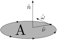
 is a line integral along the boundary of the area in question, and |A| is the magnitude of the area. If
  is an outward pointing in-plane normal, whereas is the unit-vector perpendicular to the plane (see caption at right), then the orientation of C is chosen so that a vector
  tangent to C is positively oriented if and only if
  forms a positively oriented basis for R3 (right-hand rule).
The above formula means that the curl of a vector field is defined as the infinitesimal area density of the circulation of that field. To this definition fit naturally (i) the Kelvin-Stokes theorem, as a global formula corresponding to the definition, and (ii) the following "easy to memorize" definition of the curl in orthogonal curvilinear coordinates, e.g. in cartesian coordinates, spherical, or cylindrical, or even elliptical or parabolical coordinates:
If (x1,x2,x3) are the Cartesian coordinates and (u1,u2,u3) are the curvilinear coordinates, then
 is the length of the coordinate vector corresponding to
  . The remaining two components of curl result from cyclic index-permutation: 3,1,2 → 1,2,3 → 2,3,1.
Intuitive interpretation
Suppose the vector field describes the velocity field of a fluid flow (maybe a large tank of water or gas) and a small ball is located within the fluid or gas (the centre of the ball being fixed at a certain point). If the ball has a rough surface, the fluid flowing past it will make it rotate. The rotation axis (oriented according to the right hand rule) points in the direction of the curl of the field at the centre of the ball, and the angular speed of the rotation is half the value of the curl at this point.[3]
Usage
In practice, the above definition is rarely used because in virtually all cases, the curl operator can be applied using some set of curvilinear coordinates, for which simpler representations have been derived.
The notation ∇×F has its origins in the similarities to the 3 dimensional cross product, and it is useful as a mnemonic in Cartesian coordinates if we take ∇ as a vector differential operator del. Such notation involving operators is common in physics and algebra. If certain coordinate systems are used, for instance, polar-toroidal coordinates (common in plasma physics) using the notation ∇×F will yield an incorrect result.
Expanded in Cartesian coordinates (see: Del in cylindrical and spherical coordinates for spherical and cylindrical coordinate representations), ∇×F is, for F composed of [Fx, Fy, Fz]:
where i, j, and k are the unit vectors for the x-, y-, and z-axes, respectively. This expands as follows:[4]
Although expressed in terms of coordinates, the result is invariant under proper rotations of the coordinate axes but the result inverts under reflection.
In a general coordinate system, the curl is given by[2]
where ε denotes the Levi-Civita symbol, the metric tensor is used to lower the index on F, and the Einstein summation convention implies that repeated indices are summed over. Equivalently,
where ek are the coordinate vector fields. Equivalently, using the exterior derivative, the curl can be expressed as:
Here
 and
and  are the musical isomorphisms, and
  is the Hodge dual. This formula shows how to calculate the curl of F in any coordinate system, and how to extend the curl to any oriented three dimensional Riemannian manifold. Since this depends on a choice of orientation, curl is a chiral operation. In other words, if the orientation is reversed, then the direction of the curl is also reversed.
Examples
A simple vector field
Take the vector field, which depends on x and y linearly:
Its plot looks like this:
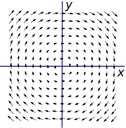
Simply by visual inspection, we can see that the field is rotating. If we place a paddle wheel anywhere, we see immediately its tendency to rotate clockwise. Using the right-hand rule, we expect the curl to be into the page. If we are to keep a right-handed coordinate system, into the page will be in the negative z direction. The lack of x and y directions is analogous to the cross product operation.
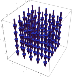
If we calculate the curl:
Which is indeed in the negative z direction, as expected. In this case, the curl is actually a constant, irrespective of position. The "amount" of rotation in the above vector field is the same at any point (x, y). Plotting the curl of F is not very interesting:
A more involved example
Suppose we now consider a slightly more complicated vector field:
Its plot:
We might not see any rotation initially, but if we closely look at the right, we see a larger field at, say, x=4 than at x=3. Intuitively, if we placed a small paddle wheel there, the larger "current" on its right side would cause the paddlewheel to rotate clockwise, which corresponds to a curl in the negative z direction. By contrast, if we look at a point on the left and placed a small paddle wheel there, the larger "current" on its left side would cause the paddlewheel to rotate counterclockwise, which corresponds to a curl in the positive z direction. Let's check out our guess by doing the math:
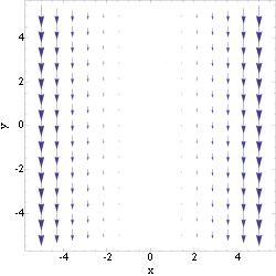
Indeed the curl is in the positive z direction for negative x and in the negative z direction for positive x, as expected. Since this curl is not the same at every point, its plot is a bit more interesting:
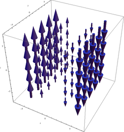
We note that the plot of this curl has no dependence on y or z (as it shouldn't) and is in the negative z direction for positive x and in the positive z direction for negative x.
Identities
Main article: Vector calculus identitiesConsider the example ∇ × [ v × F ]. Using Cartesian coordinates, it can be shown that
In the case where the vector field v and ∇ are interchanged:
which introduces the Feynman subscript notation ∇F, which means the subscripted gradient operates only on the factor F.
Another example is ∇ × [ ∇ × F ]. Using Cartesian coordinates, it can be shown that:
which can be construed as a special case of the previous example with the substitution v → ∇.
(Note:
 represents, in the case, the vector formed by the individual laplacian of each component of the vector in question)
The curl of the gradient of any scalar field is always the zero vector:
If φ is a scalar valued function and F is a vector field, then
Descriptive examples
- In a vector field describing the linear velocities of each part of a rotating disk, the curl has the same value at all points.
- Of the four Maxwell's equations, two—Faraday's law and Ampère's law—can be compactly expressed using curl. Faraday's law states that the curl of an electric field is equal to the opposite of the time rate of change of the magnetic field, while Ampère's law relates the curl of the magnetic field to the current and rate of change of the electric field.
Generalizations
The vector calculus operations of grad, curl, and div are most easily generalized and understood in the context of differential forms, which involves a number of steps. In a nutshell, they correspond to the derivatives of 0-forms, 1-forms, and 2-forms, respectively. The geometric interpretation of curl as rotation corresponds to identifying bivectors (2-vectors) in 3 dimensions with the special orthogonal Lie algebra so3 of infinitesimal rotations (in coordinates, skew-symmetric 3×3 matrices), while representing rotations by vectors corresponds to identifying 1-vectors (equivalently, 2-vectors) and so3, these all being 3-dimensional spaces.
Differential forms
Main article: Differential formIn 3 dimensions, a differential 0-form is simply a function f(x,y,z); a differential 1-form is a linear combination of three functions
 a differential 2-form is a linear combination of three functions
  and a differential 3-form is defined by a single function:
  The exterior derivative of a k-form is a (k + 1)-form, and denoting the space of k-forms by
  and the exterior derivative by d yields a sequence:
Here
 is the space of sections of the exterior algebra
  vector bundle over Rn, whose dimension is the binomial coefficient
  note that
  for k > 3 or k < 0. Writing only dimensions, one obtains a row of Pascal's triangle:
the 1-dimensional fibers correspond to functions, and the 3-dimensional fibers to vector fields, as described below. Note that modulo suitable identifications, the three nontrivial occurrences of the exterior derivative correspond to grad, curl, and div.
Differential forms and the differential can be defined on any Euclidean space, or indeed any manifold, without any notion of a Riemannian metric. On a Riemannian manifold, or more generally pseudo-Riemannian manifold, k-forms can be identified with k-vector fields (k-forms are k-covector fields, and a pseudo-Riemannian metric gives an isomorphism between vectors and covectors), and on an oriented vector space with a nondegenerate form (an isomorphism between vectors and covectors), there is an isomorphism between k-vectors and (n − k)-vectors; in particular on (the tangent space of) an oriented pseudo-Riemannian manifold. Thus on an oriented pseudo-Riemannian manifold, one can interchange k-forms, k-vector fields, (n − k)-forms, and (n − k)-vector fields; this is known as Hodge duality. Concretely, on
 this is given by:
- 1-forms and 1-vector fields: the 1-form
 corresponds to the vector field (fx,fy,fz).
 - 1-forms and 2-forms: one replaces dx by
 (i.e., omit dx), and likewise, taking care of orientation: dy corresponds to
  and dz corresponds to
  Thus corresponds to
Thus, identifying 0-forms and 3-forms with functions, and 1-forms and 2-forms with vector fields:
- grad takes a function (0-form) to a vector field (1-form);
- curl takes a vector field (1-form) to a vector field (2-form);
- div takes a vector field (2-form) to a function (3-form).
Grad and div generalize to all oriented pseudo-Riemannian manifolds, with the same geometric interpretation, because the spaces of 0-forms and n-forms is always (fiberwise) 1-dimensional and can be identified with scalar functions, while the spaces of 1-forms and (n − 1)-forms are always fiberwise n-dimensional and can be identified with vector fields.
Curl does not generalize in this way to 4 or more dimensions (or down to 2 or fewer dimensions); in 4 dimensions the dimensions are
so the curl of a 1-vector field (fiberwise 4-dimensional) is a 2-vector field, which is fiberwise 6-dimensional and cannot be identified with a 1-vector field. Nor can one meaningfully go from a 1-vector field to a 2-vector field to a 3-vector field (
 ), as taking the differential twice yields zero (d2 = 0). Thus there is no curl function from vector fields to vector fields in other dimensions arising in this way.
However, one can define a curl of a vector field as a 2-vector field in general, as described below.
Curl geometrically
2-vectors correspond to the exterior power Λ2V; in the presence of an inner product, in coordinates these are the skew-symmetric matrices, which are geometrically considered as the special orthogonal Lie algebra so(V) of infinitesimal rotations. This has
 dimensions, and allows one to interpret the differential of a 1-vector field as its infinitesimal rotations. Only in 3 dimensions (or trivially in 0 dimensions) is
  which is the most elegant and common case. is In 2 dimensions the curl of a vector field is not a vector field but a function, as 2-dimensional rotations are given by an angle (a scalar - an orientation is required to choose whether one counts clockwise or counterclockwise rotations as positive); note that this is not the div, but is rather perpendicular to it. In 3 dimensions the curl of a vector field is a vector field as is familiar (in 1 and 0 dimensions the curl of a vector field is 0, because there are no non-trivial 2-vectors), while in 4 dimensions the curl of a vector field is, geometrically, at each point an element of the 6-dimensional Lie algebra so4.
Note also that the curl of a 3-dimensional vector field which only depends on 2 coordinates (say x, y) is simply a vertical vector field (in the z direction) whose magnitude is the curl of the 2-dimensional vector field, as in the examples on this page.
Considering curl as a 2-vector field (an antisymmetric 2-tensor) has been used to generalize vector calculus and associated physics to higher dimensions.[5]
See also
- Del
- Gradient
- Divergence
- Nabla in cylindrical and spherical coordinates
- Vorticity
- Cross product
- Helmholtz decomposition
Notes
- ^ Proceedings of the London Mathematical Society, March 9th, 1871
- ^ a b Weisstein, Eric W., "Curl" from MathWorld.
- ^ Gibbs, Josiah Willard; Wilson, Edwin Bidwell (1902), Vector analysis, http://books.google.com/books?id=R5IKAAAAYAAJ&printsec=frontcover
- ^ Arfken, p. 43.
- ^ Generalizing Cross Products and Maxwell's Equations to Universal Extra Dimensions, A.W. McDavid, C.D. McMullen, 2006
References
- Arfken, George B. and Hans J. Weber. Mathematical Methods For Physicists, Academic Press; 6 edition (June 21, 2005). ISBN 978-0120598762.
- Korn, Granino Arthur and Theresa M. Korn. Mathematical Handbook for Scientists and Engineers: Definitions, Theorems, and Formulas for Reference and Review. New York: Dover Publications. pp. 157–160. ISBN 0-486-41147-8.
External links
Categories:- Linear operators in calculus
- Vector calculus
- Analytic geometry


![\nabla \times \mathbf{F} = \left[ \star \left( {\mathbf d} F^\flat \right) \right]^\sharp](e/bcec66234e170579d14ec0cb01d5e0e5.png)


![{\nabla} \times \mathbf{F} =0\boldsymbol{\hat{x}}+0\boldsymbol{\hat{y}}+ \left[{\frac{\partial}{\partial x}}(-x) -{\frac{\partial}{\partial y}} y\right]\boldsymbol{\hat{z}}=-2\boldsymbol{\hat{z}}](c/6fc584dbd3e2582a855fd07e922fca7e.png)


![\nabla \times \left( \mathbf{v \times F} \right) = \left[ \left( \mathbf{ \nabla \cdot F } \right) + \mathbf{F \cdot \nabla} \right] \mathbf{v}- \left[ \left( \mathbf{ \nabla \cdot v } \right) + \mathbf{v \cdot \nabla} \right] \mathbf{F} \ .](8/0582a2a29d6889bebba496eb0e81722c.png)


Wikimedia Foundation. 2010.