- Propagator
-
This article is about Quantum field theory. For plant propagation, see Plant propagation.
Quantum field theory 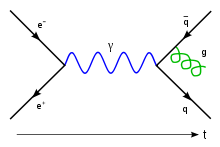
History of... BackgroundSymmetriesIncomplete theoriesScientistsJamal Nazrul Islam • Adler • Bethe • Bogoliubov • Callan • Candlin • Coleman • DeWitt • Dirac • Dyson • Fermi • Feynman • Fierz • Fröhlich • Gell-Mann • Goldstone • Gross • 't Hooft • Jackiw • Klein • Landau • Lee • Lehmann • Majorana • Nambu • Parisi • Polyakov • Salam • Schwinger • Skyrme • Stueckelberg • Symanzik • Tomonaga • Veltman • Weinberg • Weisskopf • Wilson • Witten • Yang • Yukawa • Hoodbhoy • Zimmermann • Zinn-JustinIn quantum mechanics and quantum field theory, the propagator gives the probability amplitude for a particle to travel from one place to another in a given time, or to travel with a certain energy and momentum. Propagators are used to represent the contribution of virtual particles on the internal lines of Feynman diagrams. They also can be viewed as the inverse of the wave operator appropriate to the particle, and are therefore often called Green's functions.
Contents
Non-relativistic propagators
In non-relativistic quantum mechanics the propagator gives the amplitude for a particle to travel from one spatial point at one time to another spatial point at a later time. It is a Green's function for the Schrödinger equation. This means that if a system has Hamiltonian H then the appropriate propagator is a function K(x,t;x',t') satisfying
where Hx denotes the Hamiltonian written in terms of the x coordinates and δ(x) denotes the Dirac delta-function.
This can also be written as
where
 is the unitary time-evolution operator for the system taking states at time t to states at time t'.
Path integral in quantum mechanics
The quantum mechanical propagator may also be found by using a path integral.
where the boundary conditions of the path integral include q(t)=x, q(t')=x'. Here L denotes the Lagrangian of the system. The paths that are summed over move only forwards in time.
Using the quantum mechanical propagator
In non-relativistic quantum mechanics, the propagator lets you find the state of a system given an initial state and a time interval. The new state is given by the equation:
If K(x,t;x',t') only depends on the difference x − x' this is a convolution of the initial state and the propagator.
Propagator of Free Particle and Harmonic Oscillator
For time translational invariant system, the propagator only depends on the time difference (t-t'), thus it may be rewritten as
- K(x,t;x',t') = K(x,x';t − t').
The propagator of one-dimensional free particle, with the far-right expression obtained via saddle-point approximation[1], is then
 .
.
The propagator of one-dimensional harmonic oscillator is
 .
.
For N-dimensional case, the propagator can be simply obtained by the product
 .
.
Relativistic propagators
In relativistic quantum mechanics and quantum field theory the propagators are Lorentz invariant. They give the amplitude for a particle to travel between two spacetime points.
Scalar propagator
In quantum field theory the theory of a free (non-interacting) scalar field is a useful and simple example which serves to illustrate the concepts needed for more complicated theories. It describes spin zero particles. There are a number of possible propagators for free scalar field theory. We now describe the most common ones.
Position space
The position space propagators are Green's functions for the Klein–Gordon equation. This means they are functions G(x,y) which satisfy
where:
- x,y are two points in Minkowski spacetime.
 is the d'Alembertian operator acting on the x coordinates.
- δ(x − y) is the Dirac delta-function.
(As typical in relativistic quantum field theory calculations, we use units where the speed of light, c, is 1.)
We shall restrict attention to 4-dimensional Minkowski spacetime. We can perform a Fourier transform of the equation for the propagator being this linear obtaining
This equation can be inverted in the sense of distributions noting that the equation xf(x) = 1 has the solution
 , with
  implying the limit to zero. Below we discuss the right choice of the sign arising from causality requirements and finally we can write down for the solution
where
 is the 4-vector inner product.
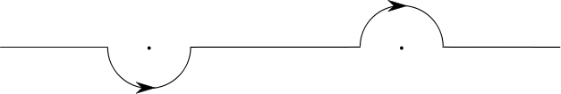
The different choices for how to deform the integration contour in the above expression lead to different forms for the propagator. The choice of contour is usually phrased in terms of the p0 integral.
The integrand then has two poles at
 so different choices of how to avoid these lead to different propagators.
Causal propagator
Retarded propagator:

A contour going clockwise over both poles gives the causal retarded propagator. This is zero if x and y are spacelike or if x0 > y0 (i.e. if x is to the future of y).
This choice of contour is equivalent to calculating the limit:
Here
is the proper time from x to y and J1 is a Bessel function of the first kind. The expression
 means x causally precedes y which, for Minkowski spacetime, means
- x0 < y0 and
 .
.
This expression can also be expressed in terms of the vacuum expectation value of the commutator of the free scalar field. Here
where

is the Heaviside step function and
is the commutator.
Advanced propagator:

A contour going anti-clockwise under both poles gives the causal advanced propagator. This is zero if x and y are spacelike or if x0 < y0 (i.e. if x is to the past of y).
This choice of contour is equivalent to calculating the limit:
This expression can also be expressed in terms of the vacuum expectation value of the commutator of the free scalar field. Here
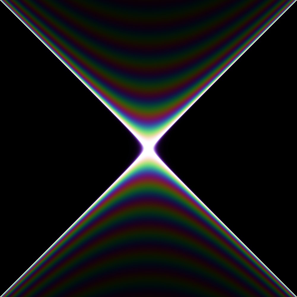
Feynman propagator
 Feynman propagator with mass 0.2. Image borders are at x = ±2 and y = ±2
 Feynman propagator with mass 2
 Feynman propagator with mass 20
 Feynman propagator with mass 200
A contour going under the left pole and over the right pole gives the Feynman propagator.
This choice of contour is equivalent to calculating the limit (see Huang p30):
Here
Here x and y are two points in Minkowski spacetime, and the dot in the exponent is a four-vector inner product.
 is a Hankel function and K1 is a modified Bessel function.
This expression can be derived directly from the field theory as the vacuum expectation value of the time-ordered product of the free scalar field, that is, the product always taken such that the time ordering of the spacetime points is the same:
This expression is Lorentz invariant as long as the field operators commute with one another when the points x and y are separated by a spacelike interval.
The usual derivation is to insert a complete set of single-particle momentum states between the fields with Lorentz covariant normalization, then show that the Θ functions providing the causal time ordering may be obtained by a contour integral along the energy axis if the integrand is as above (hence the infinitesimal imaginary part, to move the pole off the real line).
The propagator may also be derived using the path integral formulation of quantum theory.
Momentum space propagator
The Fourier transform of the position space propagators can be thought of as propagators in momentum space. These take a much simpler form than the position space propagators.
They are often written with an explicit
term although this is understood to be a reminder about which integration contour is appropriate (see above). This term is included to incorporate boundary conditions and causality (see below).For a 4-momentum p the causal and Feynman propagators in momentum space are:
For purposes of Feynman diagram calculations it is usually convenient to write these with an additional overall factor of − i (conventions vary).
Faster than light?
The Feynman propagator has some properties that seem baffling at first. In particular, unlike the commutator, the propagator is nonzero outside of the light cone, though it falls off rapidly for spacelike intervals. Interpreted as an amplitude for particle motion, this translates to the virtual particle traveling faster than light. It is not immediately obvious how this can be reconciled with causality: can we use faster-than-light virtual particles to send faster-than-light messages?
The answer is no: while in classical mechanics the intervals along which particles and causal effects can travel are the same, this is no longer true in quantum field theory, where it is commutators that determine which operators can affect one another.
So what does the spacelike part of the propagator represent? In QFT the vacuum is an active participant, and particle numbers and field values are related by an uncertainty principle; field values are uncertain even for particle number zero. There is a nonzero probability amplitude to find a significant fluctuation in the vacuum value of the field Φ(x) if one measures it locally (or, to be more precise, if one measures an operator obtained by averaging the field over a small region). Furthermore, the dynamics of the fields tend to favor spatially correlated fluctuations to some extent. The nonzero time-ordered product for spacelike-separated fields then just measures the amplitude for a nonlocal correlation in these vacuum fluctuations, analogous to an EPR correlation. Indeed, the propagator is often called a two-point correlation function for the free field.
Since, by the postulates of quantum field theory, all observable operators commute with each other at spacelike separation, messages can no more be sent through these correlations than they can through any other EPR correlations; the correlations are in random variables.
In terms of virtual particles, the propagator at spacelike separation can be thought of as a means of calculating the amplitude for creating a virtual particle-antiparticle pair that eventually disappear into the vacuum, or for detecting a virtual pair emerging from the vacuum. In Feynman's language, such creation and annihilation processes are equivalent to a virtual particle wandering backward and forward through time, which can take it outside of the light cone. However, no causality violation is involved.
Propagators in Feynman diagrams
The most common use of the propagator is in calculating probability amplitudes for particle interactions using Feynman diagrams. These calculations are usually carried out in momentum space. In general, the amplitude gets a factor of the propagator for every internal line, that is, every line that does not represent an incoming or outgoing particle in the initial or final state. It will also get a factor proportional to, and similar in form to, an interaction term in the theory's Lagrangian for every internal vertex where lines meet. These prescriptions are known as Feynman rules.
Internal lines correspond to virtual particles. Since the propagator does not vanish for combinations of energy and momentum disallowed by the classical equations of motion, we say that the virtual particles are allowed to be off shell. In fact, since the propagator is obtained by inverting the wave equation, in general it will have singularities on shell.
The energy carried by the particle in the propagator can even be negative. This can be interpreted simply as the case in which, instead of a particle going one way, its antiparticle is going the other way, and therefore carrying an opposing flow of positive energy. The propagator encompasses both possibilities. It does mean that one has to be careful about minus signs for the case of fermions, whose propagators are not even functions in the energy and momentum (see below).
Virtual particles conserve energy and momentum. However, since they can be off shell, wherever the diagram contains a closed loop, the energies and momenta of the virtual particles participating in the loop will be partly unconstrained, since a change in a quantity for one particle in the loop can be balanced by an equal and opposite change in another. Therefore, every loop in a Feynman diagram requires an integral over a continuum of possible energies and momenta. In general, these integrals of products of propagators can diverge, a situation that must be handled by the process of renormalization.
Other theories
If the particle possesses spin then its propagator is in general somewhat more complicated, as it will involve the particle's spin or polarization indices. The momentum-space propagator used in Feynman diagrams for a Dirac field representing the electron in quantum electrodynamics has the form
where the γμ are the gamma matrices appearing in the covariant formulation of the Dirac equation. It is sometimes written, using Feynman slash notation,
for short. In position space we have:
This is related to the Feynman propagator by
where
 .
.The propagator for a gauge boson in a gauge theory depends on the choice of convention to fix the gauge. For the gauge used by Feynman and Stueckelberg, the propagator for a photon is
Related singular functions
The scalar propagators are Green's functions for the Klein–Gordon equation. There are related singular functions which are important in quantum field theory. We follow the notation in Bjorken and Drell.[2] See also Bogolyubov and Shirkov (Appendix A). These function are most simply defined in terms of the vacuum expectation value of products of field operators.
Solutions to the Klein–Gordon equation
Pauli–Jordan function
The commutator of two scalar field operators defines the Pauli–Jordan function Δ(x − y) by[2]
with
This satisfies
 and is zero if (x − y)2 < 0.
Positive and negative frequency parts (cut propagators)
We can define the positive and negative frequency parts of Δ(x − y), sometimes called cut propagators, in a relativistically invariant way.
This allows us to define the positive frequency part:
 ,
,
and the negative frequency part:
 .
.
These satisfy[2]
and
Auxiliary function
The anti-commutator of two scalar field operators defines Δ1(x − y) function by
with
This satisfies

Green's functions for the Klein-Gordon equation
The retarded, advanced and Feynman propagators defined above are all Green's functions for the Klein-Gordon equation. They are related to the singular functions by[2]
where

References
- Bjorken, J.D., Drell, S.D., Relativistic Quantum Fields (Appendix C.), New York: McGraw-Hill 1965, ISBN 0-07-005494-0.
- N. N. Bogoliubov, D. V. Shirkov, Introduction to the theory of quantized fields, Wiley-Interscience, ISBN 0470086130 (Especially pp. 136–156 and Appendix A)
- Edited by DeWitt, Cécile and DeWitt, Bryce, Relativity, Groups and Topology, (Blackie and Son Ltd, Glasgow), Especially p615-624, ISBN 0444868585
- Griffiths, David J., Introduction to Elementary Particles, New York: John Wiley & Sons, 1987. ISBN 0-471-60386-4
- Halliwell, J.J., Orwitz, M. Sum-over-histories origin of the composition laws of relativistic quantum mechanics and quantum cosmology, arXiv:gr-qc/9211004
- Kerson Huang, Quantum Field Theory: From Operators to Path Integrals (New York: J. Wiley & Sons, 1998), ISBN 0-471-14120-8
- Itzykson, Claude, Zuber, Jean-Bernard Quantum Field Theory, New York: McGraw-Hill, 1980. ISBN 0-07-032071-3
- Pokorski, Stefan, Gauge Field Theories, Cambridge: Cambridge University Press, 1987. ISBN 0-521-36846-4 (Has useful appendices of Feynman diagram rules, including propagators, in the back.)
- Schulman, Larry S., Techniques & Applications of Path Integration, Jonh Wiley & Sons (New York-1981) ISBN 0471764507
- Griffith, D, Introduction to Quantum Mechanics.
External links


![K(x,t;x',t') = \int \exp \left[\frac{i}{\hbar} \int_t^{t'} L(\dot{q},q,t) dt\right] D[q(t)]](7/507b914323f020c39d2bbae3c1fd80a4.png)


![G_{ret}(x,y) = i \langle 0| \left[ \Phi(x), \Phi(y) \right] |0\rangle \Theta(x^0 - y^0)](3/2234d2d2a3b28151c87b7e75600331de.png)
![\left[\Phi(x),\Phi(y) \right]:= \Phi(x) \Phi(y) - \Phi(y) \Phi(x)](f/f5fb8066c0625817128528028837c074.png)


![G_{adv}(x,y) = -i \langle 0|\left[ \Phi(x), \Phi(y) \right]|0\rangle \Theta(y^0 - x^0).](a/2dad631d93cd61706bfcf1eefad8f482.png)


![\ = i \lang 0| [\Theta(x^0 - y^0) \Phi(x)\Phi(y) + \Theta(y^0 - x^0) \Phi(y)\Phi(x) ] |0 \rang.](c/06c38119c3ba8839fb4da68afb0f0ead.png)


![\langle 0 | \left[ \Phi(x),\Phi(y) \right] | 0 \rangle = i \Delta(x-y)](b/0cb4abb10be1b9e8059bea49db7d7304.png)


Wikimedia Foundation. 2010.