Optical flow

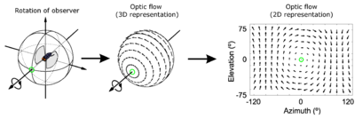The optic flow experienced by a rotating observer (in this case a fly). The direction and magnitude of optic flow at each location is represented by the direction and length of each arrow. Image taken from.^[1]

Optical flow or optic flow is the pattern of apparent motion of objects, surfaces, and edges in a visual scene caused by the relative motion between an observer (an eye or a camera) and the scene.^[2][3] The concept of optical flow was first studied in the 1940s and ultimately published by American psychologist James J. Gibson^[4] as part of his theory of affordance. Optical flow techniques such as motion detection, object segmentation, time-to-collision and focus of expansion calculations, motion compensated encoding, and stereo disparity measurement utilize this motion of the objects' surfaces and edges.^[5][6]

Estimation of the optical flow

Sequences of ordered images allow the estimation of motion as either instantaneous image velocities or discrete image displacements.^[6] Fleet and Weiss provide a tutorial introduction to gradient based optical flow .^[7] John L. Barron, David J. Fleet, and Steven Beauchemin provide a performance analysis of a number of optical flow techniques. It emphasizes the accuracy and density of measurements.^[8]

The optical flow methods try to calculate the motion between two image frames which are taken at times t and t + δt at every voxel position. These methods are called differential since they are based on local Taylor series approximations of the image signal; that is, they use partial derivatives with respect to the spatial and temporal coordinates.

For a 2D+t dimensional case (3D or n-D cases are similar) a voxel at location (x,y,t) with intensity I(x,y,t) will have moved by δx, δy and δt between the two image frames, and the following image constraint equation can be given:

I(x,y,t) = I(x + δx,y + δy,t + δt)

Assuming the movement to be small, the image constraint at I(x,y,t) with Taylor series can be developed to get:

$I(x+\delta x,y+\delta y,t+\delta t) = I(x,y,t) + \frac{\partial I}{\partial x}\delta x+\frac{\partial I}{\partial y}\delta y+\frac{\partial I}{\partial t}\delta t+$H.O.T.

From these equations it follows that:

$\frac{\partial I}{\partial x}\delta x+\frac{\partial I}{\partial y}\delta y+\frac{\partial I}{\partial t}\delta t = 0$

or

$\frac{\partial I}{\partial x}\frac{\delta x}{\delta t}+\frac{\partial I}{\partial y}\frac{\delta y}{\delta t}+\frac{\partial I}{\partial t}\frac{\delta t}{\delta t} = 0$

which results in

$\frac{\partial I}{\partial x}V_x+\frac{\partial I}{\partial y}V_y+\frac{\partial I}{\partial t} = 0$

where V_x,V_y are the x and y components of the velocity or optical flow of I(x,y,t) and $\tfrac{\partial I}{\partial x}$, $\tfrac{\partial I}{\partial y}$ and $\tfrac{\partial I}{\partial t}$ are the derivatives of the image at (x,y,t) in the corresponding directions. I_x,I_y and I_t can be written for the derivatives in the following.

Thus:

I_xV_x + I_yV_y = − I_t

or

$\nabla I^T\cdot\vec{V} = -I_t$

This is an equation in two unknowns and cannot be solved as such. This is known as the aperture problem of the optical flow algorithms. To find the optical flow another set of equations is needed, given by some additional constraint. All optical flow methods introduce additional conditions for estimating the actual flow.

Methods for determining optical flow

• Phase correlation – inverse of normalized cross-power spectrum
• Block-based methods – minimizing sum of squared differences or sum of absolute differences, or maximizing normalized cross-correlation
• Differential methods of estimating optical flow, based on partial derivatives of the image signal and/or the sought flow field and higher-order partial derivatives, such as:
  • Lucas–Kanade method – regarding image patches and an affine model for the flow field
  • Horn–Schunck method – optimizing a functional based on residuals from the brightness constancy constraint, and a particular regularization term expressing the expected smoothness of the flow field
  • Buxton–Buxton method – based on a model of the motion of edges in image sequences^[9]
  • Black–Jepson method – coarse optical flow via correlation^[6]
  • General variational methods – a range of modifications/extensions of Horn–Schunck, using other data terms and other smoothness terms.
• Discrete optimization methods – the search space is quantized, and then image matching is addressed through label assignment at every pixel, such that the corresponding deformation minimizes the distance between the source and the target image.^[10] The optimal solution is often recovered through min-cut max-flow algorithms, linear programming or belief propagation methods.

Uses of optical flow

Motion estimation and video compression have developed as a major aspect of optical flow research. While the optical flow field is superficially similar to a dense motion field derived from the techniques of motion estimation, optical flow is the study of not only the determination of the optical flow field itself, but also of its use in estimating the three-dimensional nature and structure of the scene, as well as the 3D motion of objects and the observer relative to the scene.

Optical flow was used by robotics researchers in many areas such as: object detection and tracking, image dominant plane extraction, movement detection, robot navigation and visual odometry.^[5] Optical flow information has been recognized as being useful for controlling micro air vehicles.^[11]

The application of optical flow includes the problem of inferring not only the motion of the observer and objects in the scene, but also the structure of objects and the environment. Since awareness of motion and the generation of mental maps of the structure of our environment are critical components of animal (and human) vision, the conversion of this innate ability to a computer capability is similarly crucial in the field of machine vision.^[12]

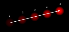The optical flow vector of a moving object in a video sequence.

Consider a five-frame clip of a ball moving from the bottom left of a field of vision, to the top right. Motion estimation techniques can determine that on a two dimensional plane the ball is moving up and to the right and vectors describing this motion can be extracted from the sequence of frames. For the purposes of video compression (e.g., MPEG), the sequence is now described as well as it needs to be. However, in the field of machine vision, the question of whether the ball is moving to the right or if the observer is moving to the left is unknowable yet critical information. Not even if a static, patterned background were present in the five frames, could we confidently state that the ball was moving to the right, because the pattern might have an infinite distance to the observer.

See also

• Optical flow sensor
• Optical mouse

References

1. ^ Huston SJ, Krapp HG (2008). Kurtz, Rafael. ed. "Visuomotor Transformation in the Fly Gaze Stabilization System". PLoS Biology 6 (7): e173. doi:10.1371/journal.pbio.0060173. PMC 2475543. PMID 18651791. http://www.plosbiology.org/article/info:doi/10.1371/journal.pbio.0060173. 
2. ^ Andrew Burton and John Radford (1978). Thinking in Perspective: Critical Essays in the Study of Thought Processes. Routledge. ISBN 0416858406. http://books.google.com/?id=CSgOAAAAQAAJ&pg=PA77&dq=%22optical+flow%22+%22optic+flow%22+date:0-1985. 
3. ^ David H. Warren and Edward R. Strelow (1985). Electronic Spatial Sensing for the Blind: Contributions from Perception. Springer. ISBN 9024726891. http://books.google.com/?id=-I_Hazgqx8QC&pg=PA414&dq=%22optical+flow%22+%22optic+flow%22+date:0-1985. 
4. ^ Gibson, J.J. (1950). The Perception of the Visual World. Houghton Mifflin. 
5. ^ ^{a b} Kelson R. T. Aires, Andre M. Santana, Adelardo A. D. Medeiros (2008). Optical Flow Using Color Information. ACM New York, NY, USA. ISBN 978-1-59593-753-7. http://delivery.acm.org/10.1145/1370000/1364064/p1607-aires.pdf?key1=1364064&key2=4460403121&coll=GUIDE&dl=GUIDE&CFID=72158298&CFTOKEN=85078203. 
6. ^ ^{a b c} S. S. Beauchemin , J. L. Barron (1995). The computation of optical flow. ACM New York, USA. http://portal.acm.org/ft_gateway.cfm?id=212141&type=pdf&coll=GUIDE&dl=GUIDE&CFID=72158298&CFTOKEN=85078203. 
7. ^ David J. Fleet and Yair Weiss (2006). "Optical Flow Estimation". In Paragios et al.. Handbook of Mathematical Models in Computer Vision. Springer. ISBN 0387263713. http://www.cs.toronto.edu/~fleet/research/Papers/flowChapter05.pdf. 
8. ^ John L. Barron, David J. Fleet, and Steven Beauchemin (1994). "Performance of optical flow techniques". International Journal of Computer Vision (Springer). http://www.cs.toronto.edu/~fleet/research/Papers/ijcv-94.pdf. 
9. ^ Glyn W. Humphreys and Vicki Bruce (1989). Visual Cognition. Psychology Press. ISBN 0863771246. http://books.google.com/?id=NiQXkMbx-lUC&pg=PA107&dq=optical-flow+Buxton-and-Buxton. 
10. ^ B. Glocker, N. Komodakis, G. Tziritas, N. Navab & N. Paragios (2008). Dense Image Registration through MRFs and Efficient Linear Programming. Medical Image Analysis Journal. http://www.mas.ecp.fr/vision/Personnel/nikos/pub/mian08.pdf. 
11. ^ Barrows G.L., Chahl J.S., and Srinivasan M.V., Biologically inspired visual sensing and flight control, Aeronautical Journal vol. 107, pp. 159–268, 2003.
12. ^ Christopher M. Brown (1987). Advances in Computer Vision. Lawrence Erlbaum Associates. ISBN 0898596483. http://books.google.com/?id=c97huisjZYYC&pg=PA133&dq=%22optic+flow%22++%22optical+flow%22. 

External links

• Finding Optic Flow
• Art of Optical Flow article on fxguide.com (using optical flow in Visual Effects)
• Optical flow evaluation and ground truth sequences.
• Middlebury Optical flow evaluation and ground truth sequences.
• mrf-registration.net - Optical flow estimation through MRF
• The French Aerospace Lab : GPU implementation of a Lucas-Kanade based optical flow
• CUDA Implementation by CUVI (CUDA Vision & Imaging Library)