Analytic signal

Not to be confused with Analytic function.

In mathematics and signal processing, the analytic representation of a real-valued function or signal facilitates many mathematical manipulations of the signal. The basic idea is that the negative frequency components of the Fourier transform (or spectrum) of a real-valued function are superfluous, due to the Hermitian symmetry of such a spectrum. These negative frequency components can be discarded with no loss of information, providing one is willing to deal with a complex-valued function instead. That makes certain attributes of the signal more accessible and facilitate the derivation of modulation and demodulation techniques, especially single-sideband. As long as the manipulated function has no negative frequency components (that is, it is still analytic), the conversion from complex back to real is just a matter of discarding the imaginary part. The analytic representation is a generalization of the phasor concept:^{[citation needed]} while the phasor is restricted to time-invariant amplitude, phase, and frequency, the analytic signal allows for time-variable parameters.

Definition

Transfer function to create an analytic signal

If x(t) is a real-valued signal with Fourier transform X(f), and u(f) is the Heaviside step function, then the function:

$\begin{align} X_\mathrm{a}(f) & \ \stackrel{\mathrm{def}}{=}\ \begin{cases} \ \ 2 X(f), & \mbox{for } f > 0, \\ \ \ X(f), & \mbox{for } f = 0, \\ \ \ 0, & \mbox{for } f < 0, \end{cases} \\ &= X(f)\cdot 2 \mathrm{u}(f) \end{align}$

contains only the non-negative frequency components of X(f). And the operation is reversible, due to the Hermitian property of X(f):

$X(f) = \begin{cases} \ \ {1 \over 2} X_\mathrm{a}(f), & \mbox{for } f > 0,\\ \ \ X^*(|f|), & \mbox{for } f < 0. \quad \quad \mbox{complex conjugate} \end{cases}$

The inverse Fourier transform of $X_\mathrm{a}(f)\,$ is the analytic signal:

$\begin{align} x_\mathrm{a}(t) &= \underbrace{\mathcal{F}^{-1}\{X(f)\}}_{x(t)} \ * \ \underbrace{\mathcal{F}^{-1}\{2 \mathrm{u}(f)\}}_{\delta(t) + j\cdot {1 \over \pi t}} \quad \quad \mbox{convolution} \\ &= x(t) + j\underbrace{\left[x(t) * {1 \over \pi t}\right]}_{\hat{x}(t)}, \end{align}$

where $\hat{x}(t)\,$ is the Hilbert transform of $x(t),\,$ and $j\,$ is the imaginary unit.

Example 1:  $x(t) = \cos(\omega_0 t)\,$, for some real parameter $\omega_0 > 0\,$

$\hat{x}(t) = \cos(\omega_0 t -\begin{matrix} \frac{\pi }{2} \end{matrix}) = \sin(\omega_0 t)\,$

$x_\mathrm{a}(t) = \cos(\omega_0 t) + j\cdot \sin(\omega_0 t) = e^{j \omega_0 t}\,$   (The 2nd equality is Euler's formula.)

This is a complex-valued signal with increasing phase (positive frequency).

It also follows from Euler's formula that $\cos(\omega_0 t) = \begin{matrix} \frac{1}{2} \end{matrix}(e^{j \omega_0 t}+e^{-j \omega_0 t}).\,$   So $x(t)\,$ comprises both positive and negative frequency components.  $x_\mathrm{a}(t)\,$ is just the positive portion. When dealing with simple sinusoids or sums of sinusoids, we can deduce $x_\mathrm{a}(t)\,$ directly, without determining $\hat{x}(t)$ first.

Example 2:  $x(t) = \cos(\omega t+\theta) = \begin{matrix} \frac{1}{2} \end{matrix} (e^{j (\omega t+\theta)} + e^{-j (\omega t+\theta)})$

$x_\mathrm{a}(t) = \begin{cases} \ \ e^{j |\omega| t}\cdot e^{j\theta} , & \mbox{if} \ \omega > 0, \\ \ \ e^{j |\omega| t}\cdot e^{-j\theta} , & \mbox{if} \ \omega < 0. \end{cases}$

The removal of the negative frequency terms is also demonstrated in Example 3. We note that nothing prevents us from computing $x_\mathrm{a}(t)\,$ for a complex-valued $x(t).\,$  But it might not be a reversible representation, because the original spectrum is not symmetrical in general. So except for this example, the general discussion assumes real-valued $x(t).\,$

Example 3:  $x(t) = e^{-j \omega_0 t}\,$, for some real parameter $\omega_0 > 0\,$

$\hat{x}(t) = j\cdot e^{-j \omega_0 t}\,$

$x_\mathrm{a}(t) = e^{-j \omega_0 t} + j^2\cdot e^{-j \omega_0 t} = 0\,$

Analytic signals are often shifted in frequency (down-converted) toward 0 Hz, which creates [non-symmetrical] negative frequency components. One motive is to allow lowpass filters with real coefficients to be used to limit the bandwidth of the signal. Another motive is to reduce the highest frequency, which reduces the minimum rate for alias-free sampling. A frequency shift does not undermine the mathematical tractability of the complex signal representation. So in that sense, the down-converted signal is still "analytic". However, restoring the real-valued representation is no longer a simple matter of just extracting the real component. Up-conversion is obviously required, and if the signal has been sampled (discrete-time), interpolation (upsampling) might also be necessary to avoid aliasing.

The complex conjugate of an analytic signal contains only negative frequency components. In that case also, there is no loss of information or reversibility by discarding the imaginary component. Obviously the real component of the complex conjugate is the same as the real component of the analytic signal. But in this case, its extraction restores the suppressed positive frequency components.

Another way to achieve a spectrum of negative frequencies is to frequency-shift the analytic signal sufficiently far in the negative direction. Extracting the real component again restores the positive frequencies. But in this case their order is reversed... the low-frequency component is now the high one. This can be used to demodulate a type of single sideband signal called lower sideband or inverted sideband.

Applications

The analytic signal can also be expressed in terms of complex polar coordinates,  $x_\mathrm{a}(t) = A(t)e^{j\phi(t)},\,$  where:

$A(t) = |x_\mathrm{a}(t)| = \sqrt { x^2(t) + \hat{x}^2(t) }\,$

$\phi(t) = \arg \left\{ x_\mathrm{a}(t) \right\}.\,$     (see arg function)

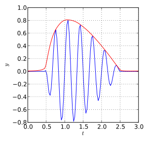A signal in blue and the magnitude of its analytic signal in red, showing the envelope effect

These functions are respectively called the amplitude envelope and instantaneous phase of the signal $x(t).\,$  In the accompanying diagram, the blue curve depicts $x(t),\,$ and the red curve depicts the corresponding $A(t).\,$
The time derivative of the unwrapped instantaneous phase is called the instantaneous frequency:.^[1]

$\omega(t) \ \stackrel{\mathrm{def}}{=}\ \phi '(t) = \frac{d}{dt} \phi(t).\,$

The amplitude function, and the instantaneous phase and frequency are in some applications used to measure and detect local features of the signal. Another application of the analytic representation of a signal relates to demodulation of modulated signals. The polar coordinates conveniently separate the effects of amplitude modulation and phase (or frequency) modulation, and effectively demodulates certain kinds of signals.

The analytic signal can also be represented as:

$x_\mathrm{a}(t)\,$	$= \left[ A(t) e^{j\phi(t)} e^{-j \omega_0 t} \right] \ e^{j \omega_0 t}$
	$= \gamma (t)\cdot e^{j \omega_0 t},$

where

$\gamma (t) = A(t)\cdot e^{j(\phi(t) - \omega_0 t)} \,$

is the signal's complex envelope. The complex envelope is not unique; on the contrary, it is determined by an arbitrary $\omega_0\,$ assignment. This concept is often used when dealing with passband signals. If $x(t)\,$ is a modulated signal, $\omega_0\,$ is usually assigned to be a carrier frequency. In other cases it is selected to be somewhere in the middle of the frequency band. Sometimes $\omega_0\,$ is chosen to minimize

$\int_{0}^{+\infty}(\omega-\omega_0)^2|X_\mathrm{a}(\omega)|^2\, d\omega.$

Alternatively [1], $\omega_0\,$ can be chosen to minimize the mean square error in linearly approximating the unwrapped instantaneous phase $\phi(t)\,$:

$\int_{-\infty}^{+\infty}(\omega(t)-\omega_0)^2 |x_\mathrm{a}(t)|^2 \, dt$

or another alternative (for some optimum $\theta \,$):

$\int_{-\infty}^{+\infty} \left( \phi(t)-(\omega_0 t + \theta) \right)^2\, dt.$.

In the field of time-frequency signal processing, it was shown that the analytic signal was needed in the definition of the Wigner-Ville Distribution so that the method can have the desirable properties needed for practical applications.^[2] More details and other applications can be found in.^[3]

Extensions of the analytic signal to signals of multiple variables

The concept of analytic signal is well-defined for signals of a single variable which typically is time. For signals of two or more variables, an analytic signal can be defined in different ways, and two approaches are presented below.

Multi-dimensional analytic signal based on an ad-hoc direction

A straightforward generalization of the analytic signal can be done for a multi-dimensional signal once it is established what is meant by negative frequencies for this case. This can be done by introducing a normalized vector $\hat{n}$ in the Fourier domain and label any frequency vector u as negative if $u \cdot \hat{n} < 0$. The analytic signal is then produced by removing all negative frequencies and multiply the result by 2, in accordance to the procedure described for the case of one-variable signals. However, there is no particular direction for $\hat{n}$ which must be chosen unless there are some additional constraints. Therefore, the choice of $\hat{n}$ is ad-hoc, or application specific.

The monogenic signal

The real and imaginary parts of the analytic signal correspond to the two elements of the vector-valued monogenic signal, as it is defined for one-variable signals. However, the monogenic signal can be extended to arbitrary number of variables in a straightforward manner, producing an (n + 1)-dimensional vector-valued function for the case of n-variable signals.

Not to be confused with

In mathematics, particularly functions of a complex variable, an analytic function refers to a function which satisfies certain properties regarding differentiability. The concept of analytic signal should not be confused with analytic functions. See the analytic representation related to the Hilbert transform for a discussion about the relation between these two concepts.

See also

• Practical considerations for computing Hilbert transforms
• Negative frequency
• Single sideband modulation (application)
• Quadrature filter (application)
• Causal filter (application)

References

1. ^ B. Boashash, "Estimating and Interpreting the Instantaneous Frequency of a Signal-Part I: Fundamentals", Proceedings of the IEEE, Vol. 80, No. 4, pp. 519-538, April 1992
2. ^ B. Boashash, “Notes on the use of the Wigner distribution for time frequency signal analysis”, IEEE Trans. on Acoust. Speech. and Signal Processing , vol. 26, no. 9, 1987
3. ^ B. Boashash, editor, "Time-Frequency Signal Analysis and Processing: A Comprehensive Reference", Elsevier Science, Oxford, 2003

• Bracewell, R; The Fourier Transform and Its Applications, 2nd ed, 1986, McGraw-Hill.
• Leon Cohen, "Time-frequency analysis", Prentice-Hall (1995)
• Frederick W. King, "Hilbert Transforms", Vol. 2, Cambridge University Press (2009).

External links

• Analytic Signals and Hilbert Transform Filters