Diffraction formalism

Main article: Diffraction

Quantitative description and analysis

For water waves propagate only on the surface of the water. The animation shows Wavelength=slitwidth blue 2D visualization

For water waves propagate only on the surface of the water. The animation shows 6*wavelength = slitwidth blue 2D visualization

Because diffraction is the result of addition of all waves (of given wavelength) along all unobstructed paths, the usual procedure is to consider the contribution of an infinitesimally small neighborhood around a certain path (this contribution is usually called a wavelet) and then integrate over all paths (=add all wavelets) from the source to the detector (or given point on a screen).

Thus in order to determine the pattern produced by diffraction, the phase and the amplitude of each of the wavelets is calculated. That is, at each point in space we must determine the distance to each of the simple sources on the incoming wavefront. If the distance to each of the simple sources differs by an integer number of wavelengths, all the wavelets will be in phase, resulting in constructive interference. If the distance to each source is an integer plus one half of a wavelength, there will be complete destructive interference. Usually, it is sufficient to determine these minima and maxima to explain the observed diffraction effects.

The simplest descriptions of diffraction are those in which the situation can be reduced to a two dimensional problem. For water waves, this is already the case, as water waves propagate only on the surface of the water. For light, we can often neglect one dimension if the diffracting object extends in that direction over a distance far greater than the wavelength. In the case of light shining through small circular holes we will have to take into account the full three dimensional nature of the problem.

General diffraction

Several qualitative observations can be made of diffraction in general:

• The angular spacing of the features in the diffraction pattern is inversely proportional to the dimensions of the object causing the diffraction. In other words: the smaller the diffracting object, the wider the resulting diffraction pattern, and vice versa. (More precisely, this is true of the sines of the angles.)
• The diffraction angles are invariant under scaling; that is, they depend only on the ratio of the wavelength to the size of the diffracting object.
• When the diffracting object has a periodic structure, for example in a diffraction grating, the features generally become sharper. The third figure, for example, shows a comparison of a double-slit pattern with a pattern formed by five slits, both sets of slits having the same spacing between the center of one slit and the next.

Approximations

The problem of calculating what a diffracted wave looks like, is the problem of determining the phase of each of the simple sources on the incoming wave front. It is mathematically easier to consider the case of far-field or Fraunhofer diffraction, where the point of observation is far from that of the diffracting obstruction, and as a result, involves less complex mathematics than the more general case of near-field or Fresnel diffraction. To make this statement more quantitative, let's consider a diffracting object at the origin that has a size $\ a$. For definiteness let's say we are diffracting light and we are interested in what the intensity looks like on a screen a distance $\ L$ away from the object. At some point on the screen the path length to one side of the object is given by the Pythagorean theorem

$S =\sqrt{L^2+(x+a/2)^2}$

If we now consider the situation where $\ L>>(x+a/2)$, the path length becomes

$S\approx(L+\frac{(x+a/2)^2}{2 L})= L + \frac{x^2}{2L}+\frac{x a}{2L}+\frac{a^2}{8L}$

This is the Fresnel approximation. To further simplify things: If the diffracting object is much smaller than the distance $\ L$, the last term will contribute much less than a wavelength to the path length, and will then not change the phase appreciably. That is $\frac{a^2}{L}<<\lambda$. The result is the Fraunhofer approximation, which is only valid very far away from the object

$S \approx L + \frac{x^2}{2L}+\frac{x a}{2L}$

Depending on the size of the diffraction object, the distance to the object and the wavelength of the wave, the Fresnel approximation, the Fraunhofer approximation or neither approximation may be valid. As the distance between the measured point of diffraction and the obstruction point increases, the diffraction patterns or results predicted converge towards those of Fraunhofer diffraction, which is more often observed in nature due to the extremely small wavelength of visible light.

Diffraction from an array of narrow slits

A simple quantitative description

Diagram of a two slit diffraction problem, showing the angle to the first minimum, where a path length difference of a half wavelength causes destructive interference.

Multiple-slit arrangements can be mathematically considered as multiple simple wave sources, if the slits are narrow enough. For light, a slit is an opening that is infinitely extended in one dimension, and this has the effect of reducing a wave problem in 3D-space to a simpler problem in 2D-space. The simplest case is that of two narrow slits, spaced a distance $\ a$ apart. To determine the maxima and minima in the amplitude we must determine the path difference to the first slit and to the second one. In the Fraunhofer approximation, with the observer far away from the slits, the difference in path length to the two slits can be seen from the image to be

$\ \Delta S={a} \sin \theta$

Maxima in the intensity occur if this path length difference is an integer number of wavelengths.

$\ {a} \sin \theta = n \lambda$		where $\ n$ is an integer that labels the order of each maximum, $\ \lambda$ is the wavelength, $\ a$ is the distance between the slits and $\ \theta$ is the angle at which constructive interference occurs.

The corresponding minima are at path differences of an integer number plus one half of the wavelength:

${a} \sin \theta = \lambda (n+1/2) \,$.

For an array of slits, positions of the minima and maxima are not changed, the fringes visible on a screen however do become sharper, as can be seen in the image.

2-slit and 5-slit diffraction of red laser light

Mathematical description

To calculate this intensity pattern, one needs to introduce some more sophisticated methods. The mathematical representation of a radial wave is given by

$\ E(r) = A \cos (k r - \omega t + \phi)/r$

where $\ k=\frac{2 \pi}{\lambda}$, $\ \lambda$ is the wavelength, $\ \omega$ is frequency of the wave and $\ \phi$ is the phase of the wave at the slits. The wave at a screen some distance away from the plane of the slits is given by the sum of the waves emanating from each of the slits. to make this problem a little easier, we introduce the complex wave $\ \Psi$, the real part of which is equal to $\ E$

$\ \Psi(r)=A e^{i (k r-\omega t +\phi)}/r$

$\ E(r)=Re(\Psi(r))$

The absolute value of this function gives the wave amplitude, and the complex phase of the function corresponds to the phase of the wave. $\ \Psi$ is referred to as the complex amplitude. With $\ N$ slits, the total wave at point $\ x$ on the screen is

$E_{total}=A e^{i(-\omega t +\phi)}\sum_{n=0}^{N-1} \frac{e^{i k \sqrt{(x-n a)^2+L^2}}}{\sqrt{(x-n a)^2+L^2}}$.

Since we are for the moment only interested in the amplitude and relative phase, we can ignore any overall phase factors that are not dependent on $\ x$ or $\ n$. We approximate $\sqrt{(x-n a)^2+L^2}\approx L+ (x-na)^2/2L$. In the Fraunhofer limit we can neglect terms of order :$\frac{a^2}{2L}$ in the exponential, and any terms involving $\ a/L$ or $\ x/L$ in the denominator. The sum becomes

$\Psi=A \frac{e^{i\left( k (\frac{x^2}{2 L}+L)-\omega t +\phi\right)}}{L}\sum_{n=0}^{N-1} e^{-i k \frac{x n a}{L}}$

The sum has the form of a geometric sum and the can be evaluated to give

$\Psi=A \frac{e^{i\left( k (\frac{x^2-(N-1)ax}{2 L}+L)-\omega t +\phi\right)}}{L} \frac {\sin\left(\frac{Nkax}{2L}\right)} {\sin\left(\frac{kax}{2L}\right)}$

The intensity is given by the absolute value of the complex amplitude squared

$I(x)=\Psi \Psi^*=|\Psi|^2=I_0\left( \frac{\sin\left(\frac{Nkax}{2L}\right)}{\sin\left(\frac{kax}{2L}\right)}\right)^2$

where Ψ ^* denotes the complex conjugate of Ψ.

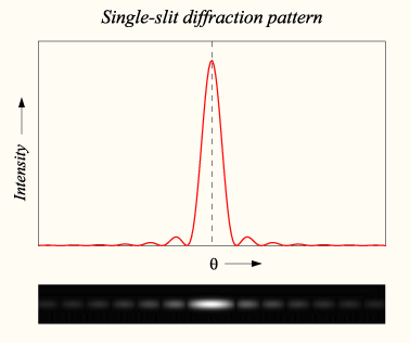
Quantitative analysis of single-slit diffraction

Numerical approximation of diffraction pattern from a slit of width equal to wavelength of an incident plane wave in 3D blue visualization

Numerical approximation of diffraction pattern from a slit of width equal to six time the wavelength of an incident plane wave in 3D blue visualization

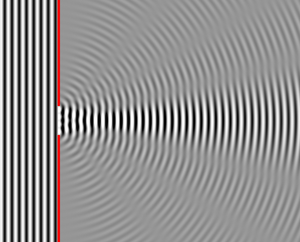Numerical approximation of diffraction pattern from a slit of width four wavelengths with an incident plane wave. The main central beam, nulls, and phase reversals are apparent.

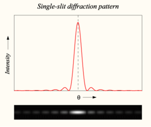Graph and image of single-slit diffraction

As an example, an exact equation can now be derived for the intensity of the diffraction pattern as a function of angle in the case of single-slit diffraction.

A mathematical representation of Huygens' principle can be used to start an equation.

Consider a monochromatic complex plane wave $\Psi^\prime$ of wavelength λ incident on a slit of width a.

If the slit lies in the x′-y′ plane, with its center at the origin, then it can be assumed that diffraction generates a complex wave ψ, traveling radially in the r direction away from the slit, and this is given by:

$\Psi = \int_{\mathrm{slit}} \frac{i}{r\lambda} \Psi^\prime e^{-ikr}\,d\mathrm{slit}$

Let (x′,y′,0) be a point inside the slit over which it is being integrated. If (x,0,z) is the location at which the intensity of the diffraction pattern is being computed, the slit extends from $x^\prime=-a/2$ to $+a/2\,$, and from $y'=-\infty$ to $\infty$.

The distance r from the slot is:

$r = \sqrt{\left(x - x^\prime\right)^2 + y^{\prime2} + z^2}$

$r = z \left(1 + \frac{\left(x - x^\prime\right)^2 + y^{\prime2}}{z^2}\right)^\frac{1}{2}$

Assuming Fraunhofer diffraction will result in the conclusion $z \gg \big|\left(x - x^\prime\right)\big|$. In other words, the distance to the target is much larger than the diffraction width on the target. By the binomial expansion rule, ignoring terms quadratic and higher, the quantity on the right can be estimated to be:

$r \approx z \left( 1 + \frac{1}{2} \frac{\left(x - x^\prime \right)^2 + y^{\prime 2}}{z^2} \right)$

$r \approx z + \frac{\left(x - x^\prime\right)^2 + y^{\prime 2}}{2z}$

It can be seen that 1/r in front of the equation is non-oscillatory, i.e. its contribution to the magnitude of the intensity is small compared to our exponential factors. Therefore, we will lose little accuracy by approximating it as 1/z.

$\Psi \,$	$= \frac{i \Psi^\prime}{z \lambda} \int_{-\frac{a}{2}}^{\frac{a}{2}}\int_{-\infty}^{\infty} e^{-ik\left[z+\frac{ \left(x - x^\prime \right)^2 + y^{\prime 2}}{2z}\right]} \,dy^\prime \,dx^\prime$
	$= \frac{i \Psi^\prime}{z \lambda} e^{-ikz} \int_{-\frac{a}{2}}^{\frac{a}{2}}e^{-ik\left[\frac{\left(x - x^\prime \right)^2}{2z}\right]} \,dx^\prime \int_{-\infty}^{\infty} e^{-ik\left[\frac{y^{\prime 2}}{2z}\right]} \,dy^\prime$
	$=\Psi^\prime \sqrt{\frac{i}{z\lambda}} e^\frac{-ikx^2}{2z} \int_{-\frac{a}{2}}^{\frac{a}{2}}e^\frac{ikxx^\prime}{z} e^\frac{-ikx^{\prime 2}}{2z} \,dx^\prime$

To make things cleaner, a placeholder 'C' is used to denote constants in the equation. It is important to keep in mind that C can contain imaginary numbers, thus the wave function will be complex. However, at the end, the ψ will be bracketed, which will eliminate any imaginary components.

Now, in Fraunhoffer diffraction, $kx^{\prime 2}/z$ is small, so $e^\frac{-ikx^{\prime 2}}{2z} \approx 1$ (note that $x^\prime$ participates in this exponential and it is being integrated).

In contrast the term $e^\frac{-ikx^2}{2z}$ can be eliminated from the equation, since when bracketed it gives 1.

$\langle e^\frac{-ikx^2}{2z}|e^\frac{-ikx^2}{2z} \rangle=e^\frac{-ikx^2}{2z} (e^\frac{-ikx^2}{2z})^*=e^\frac{-ikx^2}{2z} e^\frac{+ikx^2}{2z}=e^0=1$

(For the same reason we have also eliminated the term e ^{− ikz})

Taking $C = \Psi^\prime \sqrt{\frac{i}{z\lambda}}$ results in:

$\Psi\,$	$= C \int_{-\frac{a}{2}}^{\frac{a}{2}}e^\frac{ikxx^\prime}{z} \,dx^\prime$
	$=C \frac{\left(e^\frac{ikax}{2z} - e^\frac{-ikax}{2z}\right)}{\frac{ikx}{z}}$

It can be noted through Euler's formula and its derivatives that $\sin x = \frac{e^{ix} - e^{-ix}}{2i}$ and $\sin \theta = \frac{x}{z}$.

$\Psi = aC \frac{\sin\frac{ka\sin\theta}{2}}{\frac{ka\sin\theta}{2}} = aC \left[ \operatorname{sinc} \left( \frac{ka\sin\theta}{2} \right) \right]$

where the (unnormalized) sinc function is defined by $\operatorname{sinc}(x) \ \stackrel{\mathrm{def}}{=}\ \frac{\operatorname{sin}(x)}{x}$.

Now, substituting in $\frac{2\pi}{\lambda} = k$, the intensity (squared amplitude) I of the diffracted waves at an angle θ is given by:

$I(\theta)\,$

$= I_0 {\left[ \operatorname{sinc} \left( \frac{\pi a}{\lambda} \sin \theta \right) \right] }^2$

Quantitative analysis of N-slit diffraction

Double-slit diffraction of red laser light

2-slit and 5-slit diffraction

Let us again start with the mathematical representation of Huygens' principle.

$\Psi = \int_{\mathrm{slit}} \frac{i}{r\lambda} \Psi^\prime e^{-ikr}\,d\mathrm{slit}$

Consider N slits in the prime plane of the equal size (a, $\infty$, 0) and spacing d spread along the x′ axis. As above, the distance r from the slit 1 is:

$r = z \left(1 + \frac{\left(x - x^\prime\right)^2 + y^{\prime2}}{z^2}\right)^\frac{1}{2}$

To generalize this to N slits, we make the observation that while z and y remain constant, x′ shifts by

$x_{j=0 \cdots n-1}^{\prime} = x_0^\prime - j d$

Thus

$r_j = z \left(1 + \frac{\left(x - x^\prime - j d \right)^2 + y^{\prime2}}{z^2}\right)^\frac{1}{2}$

and the sum of all N contributions to the wave function is:

$\Psi = \sum_{j=0}^{N-1} C \int_{-\frac{a}{2}}^{\frac{a}{2}} e^\frac{ikx\left(x^\prime - jd\right)}{z} e^\frac{-ik\left(x^\prime - jd\right)^2}{2z} \,dx^\prime$

Again noting that $\frac{k\left(x^\prime -jd\right)^2}{z}$ is small, so $e^\frac{-ik\left(x^\prime -jd\right)^2}{2z} \approx 1$, we have:

$\Psi\,$	$= C\sum_{j=0}^{N-1} \int_{-\frac{a}{2}}^{\frac{a}{2}} e^\frac{ikx\left(x^\prime - jd\right)}{z} \,dx^\prime$
	$= a C \sum_{j=0}^{N-1} \frac{\left(e^{\frac{ikax}{2z} - \frac{ijkxd}{z}} - e^{\frac{-ikax}{2z}-\frac{ijkxd}{z}}\right)}{\frac{2ikax}{2z}}$
	$= a C \sum_{j=0}^{N-1} e^\frac{ijkxd}{z} \frac{\left(e^\frac{ikax}{2z} - e^\frac{-ikax}{2z}\right)}{\frac{2ikax}{2z}}$
	$= a C \frac{\sin\frac{ka\sin\theta}{2}}{\frac{ka\sin\theta}{2}} \sum_{j=1}^{N-1} e^{ijkd\sin\theta}$

Now, we can use the following identity

$\sum_{j=0}^{N-1} e^{x j} = \frac{1 - e^{Nx}}{1 - e^x}.$

Substituting into our equation, we find:

$\Psi\,$	$= a C \frac{\sin\frac{ka\sin\theta}{2}}{\frac{ka\sin\theta}{2}}\left(\frac{1 - e^{iNkd\sin\theta}}{1 - e^{ikd\sin\theta}}\right)$
	$= a C \frac{\sin\frac{ka\sin\theta}{2}}{\frac{ka\sin\theta}{2}}\left(\frac{e^{-iNkd\frac{\sin\theta}{2}}-e^{iNkd\frac{\sin\theta}{2}}}{e^{-ikd\frac{\sin\theta}{2}}-e^{ikd\frac{\sin\theta}{2}}}\right)\left(\frac{e^{iNkd\frac{\sin\theta}{2}}}{e^{ikd\frac{\sin\theta}{2}}}\right)$
	$= a C \frac{\sin\frac{ka\sin\theta}{2}}{\frac{ka\sin\theta}{2}}\frac{\frac{e^{-iNkd \frac{\sin\theta}{2}} - e^{iNkd\frac{\sin\theta}{2}}}{2i}}{\frac{e^{-ikd\frac{\sin\theta}{2}} - e^{ikd\frac{\sin\theta}{2}}}{2i}} \left(e^{i(N-1)kd\frac{\sin\theta}{2}}\right)$
	$= a C \frac{\sin\left(\frac{ka\sin\theta}{2}\right)}{\frac{ka\sin\theta}{2}} \frac{\sin\left(\frac{Nkd\sin\theta}{2}\right)} {\sin\left(\frac{kd\sin\theta}{2}\right)}e^{i\left(N-1\right)kd\frac{\sin\theta}{2}}$

We now make our k substitution as before and represent all non-oscillating constants by the I₀ variable as in the 1-slit diffraction and bracket the result. Remember that

$\langle e^{ix} \Big| e^{ix}\rangle\ = e^0 = 1$

This allows us to discard the tailing exponent and we have our answer:

$I\left(\theta\right) = I_0 \left[ \operatorname{sinc} \left( \frac{\pi a}{\lambda} \sin \theta \right) \right]^2 \cdot \left[\frac{\sin\left(\frac{N\pi d}{\lambda}\sin\theta\right)}{\sin\left(\frac{\pi d}{\lambda}\sin\theta\right)}\right]^2$

General case for far field

In the far field, where r is essentially constant, then the equation:

$\Psi = \int_{\mathrm{slit}} \frac{i}{r\lambda} \Psi^\prime e^{-ikr}\,d\mathrm{slit}$

is equivalent to doing a fourier transform on the gaps in the barrier.^[1]

See also

• diffraction grating
• Fourier analysis
• Radio telescopes

References

1. ^ [1]