- Lambert W function
-
 The graph of W(x) for W > −4 and x < 6. The upper branch with W ≥ −1 is the function W0 (principal branch), the lower branch with W ≤ −1 is the function W−1.
In mathematics, the Lambert W function, also called the Omega function or product logarithm, is a set of functions, namely the branches of the inverse relation of the function f(w) = wew where ew is the exponential function and w is any complex number. In other words, the defining equation for W(z) is
- z = W(z)eW(z)
for any complex number z.
Since the function ƒ is not injective, the relation W is multivalued (except at 0). If we restrict attention to real-valued W then the relation is defined only for x ≥ −1/e, and is double-valued on (−1/e, 0); the additional constraint W ≥ −1 defines a single-valued function W0(x). We have W0(0) = 0 and W0(−1/e) = −1. Meanwhile, the lower branch has W ≤ −1 and is denoted W−1(x). It decreases from W−1(−1/e) = −1 to W−1(0−) = −∞.
The Lambert W relation cannot be expressed in terms of elementary functions. It is useful in combinatorics, for instance in the enumeration of trees. It can be used to solve various equations involving exponentials (e.g. the maxima of the Planck, Bose-Einstein, and Fermi-Dirac distributions) and also occurs in the solution of delay differential equations, such as y'(t) = a y(t − 1).
-
 Main branch of the Lambert W function in the complex plane. Note the branch cut along the negative real axis, ending at −1/e. In this picture, the hue of a point z is determined by the argument of W(z) and the brightness by the absolute value of W(z).
Contents
Terminology
The Lambert W-function is named after Johann Heinrich Lambert. The main branch W0 is denoted by Wp in the Digital Library of Mathematical Functions and the branch W−1 is denoted by Wm there.
The notation convention chosen here (with W0 and W−1) follows the canonical reference on the Lambert-W function by Corless, Gonnet, Hare, Jeffrey and Knuth.[1]
History
Lambert first considered the related Lambert's Transcendental Equation in 1758,[2] which led to a paper by Leonhard Euler in 1783[3] that discussed the special case of wew. However the inverse of wew was first described by Pólya and Szegő in 1925.[4] The Lambert W function was "re-discovered" every decade or so in specialized applications but its full importance was not realized until the 1990s. When it was reported that the Lambert W function provides an exact solution to the quantum-mechanical double-well Dirac delta function model for equal charges—a fundamental problem in Physics—Corless and developers of the Maple Computer algebra system made a library search to find that this function was in fact ubiquitous to nature.[5]
Calculus
Derivative
By implicit differentiation, one can show that all branches of W satisfy the differential equation
(W is not differentiable for z=−1/e.) As a consequence, we get the following formula for the derivative of W:
Furthermore we have
Antiderivative
The function W(x), and many expressions involving W(x), can be integrated using the substitution w = W(x), i.e. x = w ew:
Taylor series
The Taylor series of W0 around 0 can be found using the Lagrange inversion theorem and is given by
The radius of convergence is 1/e, as may be seen by the ratio test. The function defined by this series can be extended to a holomorphic function defined on all complex numbers with a branch cut along the interval (−∞, −1/e]; this holomorphic function defines the principal branch of the Lambert W function.
Integer and complex powers
Integer powers of W0 also admit simple Taylor (or Laurent) series expansions at 0
More generally, for
 , the Lagrange inversion formula gives
which is, in general, a Laurent series of order r. Equivalently, the latter can be written in the form of a Taylor expansion of powers of W0(x) / x
which holds for any
 and | x | < e − 1.
Special values


 (the Omega constant)


Other formulas
Applications
Many equations involving exponentials can be solved using the W function. The general strategy is to move all instances of the unknown to one side of the equation and make it look like Y = XeX at which point the W function provides the value of the variable in X.
In other words :
Examples
- Example 1
More generally, the equation
where
can be transformed via the substitution
into
giving
which yields the final solution
- Example 2
Similar techniques show that
has solution
or, equivalently,
- Example 3
Whenever the complex infinite exponential tetration
converges, the Lambert W function provides the actual limit value as
where ln(z) denotes the principal branch of the complex log function.
- Example 4
Solutions for
have the form
- Example 5
The solution for the current in a series diode/resistor circuit can also be written in terms of the Lambert W. See diode modeling.
- Example 6
The delay differential equation
has characteristic equation λ = ae − λ, leading to λ = Wk(a) and
 , where k is the branch index. If a is real, only W0(a) need be considered.
- Example 7
Granular and debris flow fronts and deposits, and the fronts of viscous fluids in natural events and in the laboratory experiments can be described by using the Lambert–Euler omega function as follows:[6]
where H(x) is the debris flow height, x is the channel downstream position, L is the unified model parameter consisting of several physical and geometrical parameters of the flow, flow height and the hydraulic pressure gradient.
Generalizations
The standard Lambert W function expresses exact solutions to transcendental algebraic equations (in x) of the form:
where a0, c and r are real constants. The solution is
 . Generalizations of the Lambert W function[7] include:
- An application to general relativity and quantum mechanics (quantum gravity) in lower dimensions, in fact a previously unknown link between these two areas, as shown in Classical and Quantum Gravity where the right-hand-side of (1) is now a quadratic polynomial in x:[8]
- and where r1 and r2 are real distinct constants, the roots of the quadratic polynomial. Here, the solution is a function has a single argument x but the terms like ri and ao are parameters of that function. In this respect, the generalization resembles the hypergeometric function and the Meijer G-function but it belongs to a different class of functions. When r1 = r2, both sides of (2) can be factored and reduced to (1) and thus the solution reduces to that of the standard W function. Eq. (2) expresses the equation governing the dilaton field, from which is derived the metric of the R=T or lineal two-body gravity problem in 1+1 dimensions (one spatial dimension and one time dimension) for the case of unequal (rest) masses, as well as, the eigenenergies of the quantum-mechanical double-well Dirac delta function model for unequal charges in one dimension.
- Analytical solutions of the eigenenergies of a special case of the quantum mechanical three-body problem, namely the (three-dimensional) hydrogen molecule-ion.[9] Here the right-hand-side of (1) (or (2)) is now a ratio of infinite order polynomials in x:
- where ri and si are distinct real constants and x is a function of the eigenenergy and the internuclear distance R. Eq. (3) with its specialized cases expressed in (1) and (2) is related to a large class of delay differential equations.
Applications of the Lambert "W" function in fundamental physical problems are not exhausted even for the standard case expressed in (1) as seen recently in the area of atomic, molecular, and optical physics.[10]
Plots
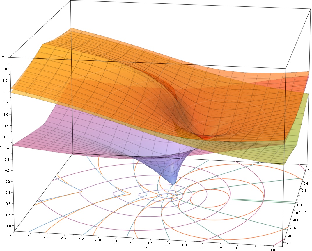
- Plots of the Lambert W function on the complex plane
-

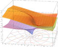
z = Re(W0(x + i y))
-

z = Im(W0(x + i y))
-
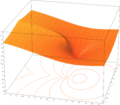
z = |W0(x + i y)|
-
Numerical evaluation
The W function may be approximated using Newton's method, with successive approximations to w = W(z) (so z = wew) being
The W function may also be approximated using Halley's method,
given in Corless et al. to compute W.
See also
- Lambert's trinomial equation
- Lagrange inversion theorem
- Experimental mathematics
- R=T model
Notes
- ^ Corless, R. M.; Gonnet, G. H.; Hare, D. E. G.; Jeffrey, D. J.; Knuth, D. E. (1996). "On the Lambert W function". Advances in Computational Mathematics 5: 329–359. doi:10.1007/BF02124750. http://www.apmaths.uwo.ca/~rcorless/frames/PAPERS/LambertW/LambertW.ps.
- ^ Lambert JH, "Observationes variae in mathesin puram", Acta Helveticae physico-mathematico-anatomico-botanico-medica, Band III, 128–168, 1758 (facsimile)
- ^ Euler, L. "De serie Lambertina Plurimisque eius insignibus proprietatibus." Acta Acad. Scient. Petropol. 2, 29–51, 1783. Reprinted in Euler, L. Opera Omnia, Series Prima, Vol. 6: Commentationes Algebraicae. Leipzig, Germany: Teubner, pp. 350–369, 1921. (facsimile)
- ^ Pólya, George; Szegő, Gábor (1998) [1925]. Aufgaben und Lehrsätze der Analysis [Problems and Theorems in Analysis]. Berlin: Springer-Verlag.
- ^ Corless, R. M.; Gonnet, G. H.; Hare, D. E. G.; Jeffrey, D. J. (1993). "Lambert's W function in Maple". The Maple Technical Newsletter (MapleTech) 9: 12–22.
- ^ Pudasaini, S.P. (2011). "Some exact solutions for debris and avalanche flows". Physics of Fluids 23 (4): 043301. doi:10.1063/1.3570532.
- ^ Scott, T. C.; Mann, R. B. (2006). "General Relativity and Quantum Mechanics: Towards a Generalization of the Lambert W Function". AAECC (Applicable Algebra in Engineering, Communication and Computing) 17 (1): 41–47. arXiv:math-ph/0607011. doi:10.1007/s00200-006-0196-1.
- ^ Farrugia, P. S.; Mann, R. B.; Scott, T. C. (2007). "N-body Gravity and the Schrödinger Equation". Class. Quantum Grav. 24 (18): 4647–4659. arXiv:gr-qc/0611144. doi:10.1088/0264-9381/24/18/006.
- ^ Scott, T. C.; Aubert-Frécon, M.; Grotendorst, J. (2006). "New Approach for the Electronic Energies of the Hydrogen Molecular Ion". Chem. Phys. 324 (2–3): 323–338. arXiv:physics/0607081. doi:10.1016/j.chemphys.2005.10.031.
- ^ Scott, T. C.; Lüchow, A.; Bressanini, D.; Morgan, J. D. III (2007). "The Nodal Surfaces of Helium Atom Eigenfunctions". Phys. Rev. A 75 (6): 060101. doi:10.1103/PhysRevA.75.060101.
References
- Corless, R.; Gonnet, G.; Hare, D.; Jeffrey, D.; Knuth, Donald (1996), "On the Lambert W function", Advances in Computational Mathematics (Berlin, New York: Springer-Verlag) 5: 329–359, ISSN 1019-7168, http://www.apmaths.uwo.ca/~djeffrey/Offprints/W-adv-cm.pdf
- Chapeau-Blondeau, F. and Monir, A: "Evaluation of the Lambert W Function and Application to Generation of Generalized Gaussian Noise With Exponent 1/2", IEEE Trans. Signal Processing, 50(9), 2002
- Francis et al. "Quantitative General Theory for Periodic Breathing" Circulation 102 (18): 2214. (2000). Use of Lambert function to solve delay-differential dynamics in human disease.
- Roy, R.; Olver, F. W. J. (2010), "Lambert W function", in Olver, Frank W. J.; Lozier, Daniel M.; Boisvert, Ronald F. et al., NIST Handbook of Mathematical Functions, Cambridge University Press, ISBN 978-0521192255, MR2723248, http://dlmf.nist.gov/4.13
- Veberic, D., "Having Fun with Lambert W(x) Function" arXiv:1003.1628 (2010). C++ implementation using Halley's and Fritsch's iteration.
External links
- National Institute of Science and Technology Digital Library - Lambert W
- MathWorld - Lambert W-Function
- Computing the Lambert W function
- Corless et al. Notes about Lambert W research
- Extreme Mathematics. Monographs on the Lambert W function, its numerical approximation and generalizations for W-like inverses of transcendental forms with repeated exponential towers.
- GPL C++ implementation with Halley's and Fritsch's iteration.
Categories:


![H(x)= 1 + W[(H(0) -1)exp((H(0)-1)-\frac{x}{L})],](9/8d9812899386275810a391783232a5a8.png)


Wikimedia Foundation. 2010.