- Mixing (mathematics)
-
In mathematics, mixing is an abstract concept originating from physics: the attempt to describe the irreversible thermodynamic process of mixing in the everyday world: mixing paint, mixing drinks, etc.The concept appears in ergodic theory—the study of stochastic processes and measure-preserving dynamical systems. Several different definitions for mixing exist, including strong mixing, weak mixing and topological mixing, with the last not requiring a measure to be defined. Some of the different definitions of mixing can be arranged in a hierarchical order; thus, strong mixing implies weak mixing. Furthermore, weak mixing (and thus also strong mixing) implies ergodicity: that is, every system that is weakly mixing is also ergodic (and so one says that mixing is a "stronger" notion than ergodicity).
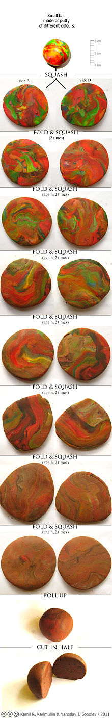 Mixing in a ball of colored putty after consecutive iterations of "Smale horseshoe map" (i.e. squashing and folding in two)
Contents
Mixing in stochastic processes
Let
 be a sequence of random variables. Such a sequence is naturally endowed with a topology, the product topology. The open sets of this topology are called cylinder sets. These cylinder sets generate a sigma algebra, the Borel sigma algebra; it is the smallest (coarsest) sigma algebra that contains the topology.
Define a function α(s), called the strong mixing coefficient, as
In this definition, P is the probability measure on the sigma algebra. The symbol
 , with
  denotes a subalgebra of the sigma algebra; it is the set of cylinder sets that are specified between times a and b. Given specific, fixed values Xa, Xa + 1, etc., of the random variable, at times a, a + 1, etc., then it may be thought of as the sigma-algebra generated by
The process
 is strong mixing if
  as
as  .
.One way to describe this is that strong mixing implies that for any two possible states of the system (realizations of the random variable), when given a sufficient amount of time between the two states, the occurrence of the states is independent.
Types of mixing
Suppose {Xt} is a stationary Markov process, with stationary distribution Q. Denote L²(Q) the space of Borel-measurable functions that are square-integrable with respect to measure Q. Also let ℰtϕ(x) = E[ϕ(Xt) | X0 = x] denote the conditional expectation operator on L²(Q). Finally, let Z = {ϕ∈L²(Q): ∫ ϕdQ = 0} denote the space of square-integrable functions with mean zero.
The ρ-mixing coefficients of the process {xt} are
The process is called ρ-mixing if these coefficients converge to zero as t → ∞, and “ρ-mixing with exponential decay rate” if ρt < e−δt for some δ > 0. For a stationary Markov process, the coefficients ρt may either decay at an exponential rate, or be always equal to one. [1]
The α-mixing coefficients of the process {xt} are
The process is called α-mixing if these coefficients converge to zero as t → ∞, it is “α-mixing with exponential decay rate” if αt < γe−δt for some δ > 0, and it is “α-mixing with sub-exponential decay rate” if αt < ξ(t) for some non-increasing function ξ(t) satisfying t−1ln ξ(t) → 0 as t → ∞. [1]
The α-mixing coefficients are always smaller than the ρ-mixing ones: αt ≤ ρt, therefore if the process is ρ-mixing, it will necessarily be α-mixing too. However when ρt = 1, the process may still be α-mixing, with sub-exponential decay rate.
The β-mixing coefficients are given by
The process is called β-mixing if these coefficients converge to zero as t → ∞, it is “β-mixing with exponential decay rate” if βt < γe−δt for some δ > 0, and it is “β-mixing with sub-exponential decay rate” if βtξ(t) → 0 as t → ∞ for some non-increasing function ξ(t) satisfying t−1ln ξ(t) → 0 as t → ∞.[1]
A strictly stationary Markov process is β-mixing if and only if it is an aperiodic recurrent Harris chain. The β-mixing coefficients are always bigger than the α-mixing ones, so if a process is β-mixing it will also be α-mixing. There is no direct relationship between β-mixing and ρ-mixing: neither of them implies the other.
Mixing in dynamical systems
A similar definition can be given using the vocabulary of measure-preserving dynamical systems. Let
 be a dynamical system, with T being the time-evolution or shift operator. The system is said to be strong mixing if, for any
  , one has
 .
.
For shifts parametrized by a continuous variable instead of a discrete integer n, the same definition applies, with T − n replaced by Tg with g being the continuous-time parameter.
To understand the above definition physically, consider a shaker M full of an incompressible liquid, which consists of 20% wine and 80% water. If A is the region originally occupied by the wine, then, for any part B of the shaker, the percentage of wine in B after n repetitions of the act of stirring is
In such a situation, one would expect that after the liquid is sufficiently stirred (
 ), every part B of the shaker will contain approximately 20% wine. This leads to
which implies the above definition of strong mixing.
A dynamical system is said to be weak mixing if one has
In other words, T is strong mixing if
 converges towards μ(A)μ(B). and weak mixing if this convergence is only in the Cesàro sense).
Weak mixing is a sufficient condition for ergodicity.
For a system that is weak mixing, the shift operator T will have no (non-constant) square-integrable eigenfunctions with associated eigenvalue of one.[citation needed] In general, a shift operator will have a continuous spectrum, and thus will always have eigenfunctions that are generalized functions. However, for the system to be (at least) weak mixing, none of the eigenfunctions with associated eigenvalue of one can be square integrable.
Topological mixing
A form of mixing may be defined without appeal to a measure, only using the topology of the system. A continuous map
 is said to be topologically transitive if, for every pair of non-empty open sets
  , there exists an integer n such that
where fn is the n 'th iterate of f. In the operator theory, a topologically transitive bounded linear operator (a continuous linear map on a topological vector space) is usually called hypercyclic operator. A related idea is expressed by the wandering set.
Lemma: If X is a compact metric space, then f is topologically transitive if and only if there exists a hypercyclic point
 , that is, a point x such that its orbit
  is dense in X.
A system is said to be topologically mixing if, given sets A and B, there exists an integer N, such that, for all n > N, one has
 .
.
For a continuous-time system, fn is replaced by the flow ϕg, with g being the continuous parameter, with the requirement that a non-empty intersection hold for all
 .
.A weak topological mixing is one that has no non-constant continuous (with respect to the topology) eigenfunctions of the shift operator.
Topological mixing neither implies, nor is implied by either weak or strong mixing: there are examples of systems that are weak mixing but not topologically mixing, and examples that are topologically mixing but not strong mixing.
Generalizations
The definition given above is sometimes called strong 2-mixing, to distinguish it from higher orders of mixing. A strong 3-mixing system may be defined as a system for which
holds for all measurable sets A, B, C. We can define strong k-mixing similarly. A system which is strong k-mixing for all k=2,3,4,... is called mixing of all orders.
It is unknown whether strong 2-mixing implies strong 3-mixing. It is known that strong m-mixing implies ergodicity.
References
- Chen, Xiaohong; Hansen, Lars Peter; Carrasco, Marine (2010). "Nonlinearity and temporal dependence". Journal of Econometrics 155 (2): 155–169. doi:10.1016/j.jeconom.2009.10.001.
- Achim Klenke, Probability Theory, (2006) Springer ISBN 978-1-84800-047-6
- V. I. Arnold and A. Avez, Ergodic Problems of Classical Mechanics, (1968) W. A. Benjamin, Inc.
Categories:- Stochastic processes
- Ergodic theory


Wikimedia Foundation. 2010.