- Directional statistics
-
Directional statistics is the subdiscipline of statistics that deals with directions (unit vectors in Rn), axes (lines through the origin in Rn) or rotations in Rn. More generally, directional statistics deals with observations on compact Riemannian manifolds.
The fact that 0 degrees and 360 degrees are identical angles, so that for example 180 degrees is not a sensible mean of 2 degrees and 358 degrees, provides one illustration that special statistical methods are required for the analysis of some types of data (in this case, angular data). Other examples of data that may be regarded as directional include statistics involving temporal periods (e.g. time of day, week, month, year, etc.), compass directions, dihedral angles in molecules, orientations, rotations and so on.
Circular and higher dimensional distributions
Any probability density function p(x) on the line can be "wrapped" around the circumference of a circle of unit radius.[2] That is, the pdf of the wrapped variable
is
This concept can be extended to the multivariate context by an extension of the simple sum to a number of F sums that cover all dimensions in the feature space:
where
 is the kth Euclidean basis vector.
Examples of circular distributions
- The von Mises distribution is a circular distribution which, like any other circular distribution, may be thought of as a wrapping of a certain linear probability distribution around the circle. The underlying linear probability distribution for the von Mises distribution is mathematically intractable, however, for statistical purposes, there is no need to deal with the underlying linear distribution. The usefulness of the von Mises distribution is twofold: it is the most mathematically tractable of all circular distributions, allowing simpler statistical analysis, and it is a close approximation to the wrapped normal distribution, which, analogously the linear normal distribution, is important because it is the limiting case for the sum of a large number of small angular deviations. In fact, the von Mises distribution is often known as the "circular normal" distribution because of its ease of use and its close relationship to the wrapped normal distribution (Fisher, 1993).
- The pdf of the von Mises distribution is:
- where I0 is the modified Bessel function of order 0.
- The pdf of the circular uniform distribution is given by
- The pdf of the wrapped normal distribution (WN) is:
-
- where μ and σ are the mean and standard deviation of the unwrapped distribution, respectively and ζ(θ,τ) is the Jacobi theta function:
-
 where
where  and
and 
- The pdf of the wrapped Cauchy distribution (WC) is:
- where γ is the scale factor and θ0 is the peak position.
- The pdf of the Wrapped Lévy distribution (WL) is:
- where the value of the summand is taken to be zero when
 , c is the scale factor and μ is the location parameter.
Distributions on higher dimensional manifolds
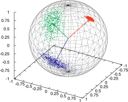 Three points sets sampled from different Kent distributions on the sphere.
There also exist distributions on the two-dimensional sphere (such as the Kent distribution[3]), the N-dimensional sphere (the Von Mises-Fisher distribution[4]) or the torus (the bivariate von Mises distribution[5]).
The matrix-von Mises–Fisher distribution is a distribution on the Stiefel manifold, and can be used to construct probability distributions over rotation matrices.[6]
The Bingham distribution is a distribution over axes in N dimensions, or equivalently, over points on the (N − 1)-dimensional sphere with the antipodes identified.[7] For example, if N = 2, the axes are undirected lines through the origin in the plane. In this case, each axis cuts the unit circle in the plane (which is the one-dimensional sphere) at two points that are each other's antipodes. For N = 4, the Bingham distribution is a distribution over the space of unit quaternions. Since a unit quaternion corresponds to a rotation matrix, the Bingham distribution for N = 4 can be used to construct probability distributions over the space of rotations, just like the Matrix-von Mises–Fisher distribution.
These distributions are for example used in geology,[8] crystallography[9] and bioinformatics.[10] [11] [12]
The fundamental difference between linear and circular statistics
A simple way to calculate the mean of a series of angles (in the interval [0°, 360°)) is to calculate the mean of the cosines and sines of each angle, and obtain the angle by calculating the inverse tangent. Consider the following three angles as an example: 10, 20, and 30 degrees. Intuitively, calculating the mean would involve adding these three angles together and dividing by 3, in this case indeed resulting in a correct mean angle of 20 degrees. By rotating this system anticlockwise through 15 degrees the three angles become 355 degrees, 5 degrees and 15 degrees. The naive mean is now 125 degrees, which is the wrong answer, as it should be 5 degrees. The vector mean
 can be calculated in the following way, using the mean sine
  and the mean cosine
  :
:This may be more succinctly stated by realizing that directional data are in fact vectors of unit length. In the case of one-dimensional data, these data points can be represented conveniently as complex numbers of unit magnitude
 , where θ is the measured angle. The mean resultant vector for the sample is then:
The sample mean angle is then the argument of the mean resultant:
The length of the sample mean resultant vector is:
and will have a value between 0 and 1. Thus the sample mean resultant vector can be represented as:
Moments
The raw vector (or trigonometric) moments of a circular distribution are defined as
where Γ is any interval of length 2π and P(θ) is the PDF of the circular distribution. Since the integral P(θ) is unity, and the integration interval is finite, it follows that the moments of any circular distribution are always finite and well defined.
Sample moments are analogously defined:
The population resultant vector, length, and mean angle are defined in analogy with the corresponding sample parameters.
In addition, the lengths of the higher moments are defined as:
while the angular parts of the higher moments are just
 . The lengths of the higher moments will all lie between 0 and 1.
Measures of location and spread
Main article: Mean of circular quantitiesVarious measures of location and spread may be defined for both the population and a sample drawn from that population.[13] The most common measure of location is the circular mean. The population circular mean is simply the first moment of the distribution while the sample mean is the first moment of the sample. The sample mean will serve as an unbiased estimator of the population mean.
When data is concentrated, the median and mode may be defined by analogy to the linear case, but for more dispersed or multi-modal data, these concepts are not useful.
The most common measures of circular spread are:
- The circular variance. For the sample the circular variance is defined as:
- and for the population
- Both will have values between 0 and 1.
- The circular standard deviation
- with values between 0 and infinity. This definition of the standard deviation (rather than the square root of the variance) is useful because for a wrapped normal distribution, it is an estimator of the standard deviation of the underlying normal distribution. It will therefore allow the circular distribution to be standardized as in the linear case, for small values of the standard deviation. This also applies to the von Mises distribution which closely approximates the wrapped normal distribution.
- The circular dispersion
- with values between 0 and infinity. This measure of spread is found useful in the statistical analysis of variance.
Distribution of the mean
Given a set of N measurements
 the mean value of z is defined as:
which may be expressed as
where
or, alternatively as:
where
The distribution of the mean (
 ) for a circular pdf P(θ) will be given by:
where Γ is over any interval of length 2π and the integral is subject to the constraint that
 and
and  are constant, or, alternatively, that
  and are constant.
The calculation of the distribution of the mean for most circular distributions is not analytically possible, and in order to carry out an analysis of variance, numerical or mathematical approximations are needed.[14]
The central limit theorem may be applied to the distribution of the sample means. (main article: Central limit theorem for directional statistics). It can be shown[15] that the distribution of
![[\overline{C},\overline{S}]](6/0e646003c8a7cb604b1fa5b82367f9e2.png) approaches a bivariate normal distribution in the limit of large sample size.
approaches a bivariate normal distribution in the limit of large sample size.Software
- R has some packages devoted to circular statistics, including CircStats. (CircStats package for R)
- Circular Statistics, a MATLAB toolbox containing the essentials to work with circular data (Documentation).
- Mocapy: a dynamic Bayesian network software package implemented in Python and C++. Uses stochastic expectation maximization for parameter learning, and supports directional statistics.
- Oriana, Windows software for directional statistics.
See also
- Yamartino method
- Wrapped distribution
References
- ^ "Hamelryck, T., Kent, J., Krogh, A. (2006) Sampling realistic protein conformations using local structural bias. PLoS Comput. Biol., 2(9): e131". Public Library of Science (PLoS). http://compbiol.plosjournals.org/perlserv/?request=get-document&doi=10.1371/journal.pcbi.0020131. Retrieved 2008-02-01.
- ^ Bahlmann, C., (2006), Directional features in online handwriting recognition, Pattern Recognition, 39
- ^ Kent, J (1982) The Fisher–Bingham distribution on the sphere. J Royal Stat Soc, 44, 71–80.
- ^ Fisher, RA (1953) Dispersion on a sphere. Proc. Roy. Soc. London Ser. A., 217, 295–305
- ^ Mardia, KM. Taylor, CC., Subramaniam, GK. (2007) Protein Bioinformatics and Mixtures of Bivariate von Mises Distributions for Angular Data. Biometrics, 63, 505–512
- ^ Downs, (1972) Orientational statistics. Biometrica, 59, 665–676
- ^ Bingham, C. (1974) An Antipodally Symmetric Distribution on the Sphere. Ann. Statist., 2, 1201-1225.
- ^ Peel, D., Whiten, WJ., McLachlan, GJ. (2001) Fitting mixtures of Kent distributions to aid in joint set identification. J. Am. Stat. Ass., 96, 56–63
- ^ Krieger Lassen, N. C., Juul Jensen, D. & Conradsen, K. (1994) On the statistical analysis of orientation data. Acta Cryst., A50, 741–748.
- ^ Kent, J.T., Hamelryck, T. (2005). Using the Fisher–Bingham distribution in stochastic models for protein structure. In S. Barber, P.D. Baxter, K.V.Mardia, & R.E. Walls (Eds.), Quantitative Biology, Shape Analysis, and Wavelets, pp. 57–60. Leeds, Leeds University Press
- ^ "Hamelryck, T., Kent, J., Krogh, A. (2006) Sampling realistic protein conformations using local structural bias. PLoS Comput. Biol., 2(9): e131". Public Library of Science (PLoS). http://compbiol.plosjournals.org/perlserv/?request=get-document&doi=10.1371/journal.pcbi.0020131. Retrieved 2008-02-01.
- ^ "Boomsma, W., Mardia, KV., Taylor, CC., Ferkinghoff-Borg, J., Krogh, A., Hamelryck, T. (2008) A generative, probabilistic model of local protein structure. Proc. Natl. Acad. Sci. USA, 105(26), 8932-8937". http://www.pnas.org/cgi/content/abstract/0801715105v1?etoc. Retrieved 2008-06-26.
- ^ Fisher, NI., Statistical Analysis of Circular Data, Cambridge University Press, 1993. ISBN 0-521-35018-2
- ^ Jammalamadaka, S. Rao; Sengupta, A. (2001). Topics in Circular Statistics. World Scientific Publishing Company. ISBN 978-9810237783. http://www.amazon.com/Topics-Circular-Statistics-Rao-Jammalamadaka/dp/9810237782#reader_9810237782. Retrieved 2010-03-03.
- ^ Jammalamadaka, S. Rao; SenGupta, A. (2001). Topics in circular statistics. New Jersey: World Scientific. ISBN 9810237782. http://books.google.com/books?id=sKqWMGqQXQkC&printsec=frontcover&dq=Jammalamadaka+Topics+in+circular&hl=en&ei=iJ3QTe77NKL00gGdyqHoDQ&sa=X&oi=book_result&ct=result&resnum=1&ved=0CDcQ6AEwAA#v=onepage&q&f=false. Retrieved 2011-05-15.
Books on directional statistics
- Batschelet, E. Circular statistics in biology, Academic Press, London, 1981. ISBN 0-12-081050-6.
- Fisher, NI., Statistical Analysis of Circular Data, Cambridge University Press, 1993. ISBN 0-521-35018-2
- Fisher, NI., Lewis, T., Embleton, BJJ. Statistical Analysis of Spherical Data, Cambridge University Press, 1993. ISBN 0-521-45699-1
- Mardia, KV. and Jupp P., Directional Statistics (2nd edition), John Wiley and Sons Ltd., 2000. ISBN 0-471-95333-4
External links
- Directional Statistics, Concepts and Techniques in Modern Geography 25
- CircStat: A MATLAB Toolbox for Circular Statistics, Journal of Statistical Software, Vol. 31, Issue 10, Sep 2009
Categories:- Statistical data types
- Statistical models
- Types of probability distributions
- Directional statistics
![\theta = x_w=x \mod 2\pi\ \ \in (-\pi,\pi]](5/ec53d92b8b1c13825019acf24bef8f5b.png)


![WN(\theta;\mu,\sigma)=\frac{1}{\sigma \sqrt{2\pi}} \sum^{\infty}_{k=-\infty} \exp \left[\frac{-(\theta - \mu - 2\pi k)^2}{2 \sigma^2} \right]=\frac{1}{2\pi}\zeta\left(\frac{\theta-\mu}{2\pi},\frac{i\sigma^2}{2\pi}\right)](a/25a2a71123a4fbae39a6dbb54dcb137e.png)


![P(\overline{C},\overline{S}) \, d\overline{C} \, d\overline{S} =
P(\overline{R},\overline{\theta}) \, d\overline{R} \, d\overline{\theta} =
\int_\Gamma ... \int_\Gamma \prod_{n=1}^N \left[ P(\theta_n) \, d\theta_n \right]](7/b77634604e27650c26c752e0aafa67eb.png)
Wikimedia Foundation. 2010.