Gaussian elimination

In linear algebra, Gaussian elimination is an algorithm for solving systems of linear equations. It can also be used to find the rank of a matrix, to calculate the determinant of a matrix, and to calculate the inverse of an invertible square matrix. The method is named after Carl Friedrich Gauss, but it was not invented by him.

Elementary row operations are used to reduce a matrix to what is called triangular form (in numerical analysis) or row echelon form (in abstract algebra). Gauss–Jordan elimination, an extension of this algorithm, reduces the matrix further to diagonal form, which is also known as reduced row echelon form. Gaussian elimination alone is sufficient for many applications, and requires fewer calculations than the Gauss–Jordan version.

History

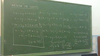Gaussian elimination

The method of Gaussian elimination appears in Chapter Eight, Rectangular Arrays, of the important Chinese mathematical text Jiuzhang suanshu or The Nine Chapters on the Mathematical Art. Its use is illustrated in eighteen problems, with two to five equations. The first reference to the book by this title is dated to 179 CE, but parts of it were written as early as approximately 150 BCE.^[1] It was commented on by Liu Hui in the 3rd century.

The method in Europe stems from the notes of Isaac Newton.^{[2] [3]} In 1670, he wrote that all the algebra books known to him lacked a lesson for solving simultaneous equations, which Newton then supplied. Cambridge University eventually published the notes as Arithmetica Universalis in 1707 long after Newton left academic life. The notes were widely imitated, which made (what is now called) Gaussian elimination a standard lesson in algebra textbooks by the end of the 18th century. Carl Friedrich Gauss in 1810 devised a notation for symmetric elimination that was adopted in the 19th century by professional hand computers to solve the normal equations of least-squares problems. The algorithm that is taught in high school was named for Gauss only in the 1950s as a result of confusion over the history of the subject.

Algorithm overview

The process of Gaussian elimination has two parts. The first part (Forward Elimination) reduces a given system to either triangular or echelon form, or results in a degenerate equation with no solution, indicating the system has no solution. This is accomplished through the use of elementary row operations. The second step uses back substitution to find the solution of the system above.

Stated equivalently for matrices, the first part reduces a matrix to row echelon form using elementary row operations while the second reduces it to reduced row echelon form, or row canonical form.

Another point of view, which turns out to be very useful to analyze the algorithm, is that Gaussian elimination computes a matrix decomposition. The three elementary row operations used in the Gaussian elimination (multiplying rows, switching rows, and adding multiples of rows to other rows) amount to multiplying the original matrix with invertible matrices from the left. The first part of the algorithm computes an LU decomposition, while the second part writes the original matrix as the product of a uniquely determined invertible matrix and a uniquely determined reduced row-echelon matrix.

Example

Suppose the goal is to find and describe the solution(s), if any, of the following system of linear equations:

$\begin{alignat}{7} 2x &&\; + \;&& y &&\; - \;&& z &&\; = \;&& 8 & \qquad (L_1) \\ -3x &&\; - \;&& y &&\; + \;&& 2z &&\; = \;&& -11 & \qquad (L_2) \\ -2x &&\; + \;&& y &&\; +\;&& 2z &&\; = \;&& -3 & \qquad (L_3) \end{alignat}$

The algorithm is as follows: eliminate x from all equations below L₁, and then eliminate y from all equations below L₂. This will put the system into triangular form. Then, using back-substitution, each unknown can be solved for.

In the example, x is eliminated from L₂ by adding $\begin{matrix}\frac{3}{2}\end{matrix} L_1$ to L₂. x is then eliminated from L₃ by adding L₁ to L₃. Formally:

$L_2 + \frac{3}{2}L_1 \rightarrow L_2$

$L_3 + L_1 \rightarrow L_3$

The result is:

$\begin{alignat}{7} 2x &&\; + && y &&\; - &&\; z &&\; = \;&& 8 & \\ && && \frac{1}{2}y &&\; + &&\; \frac{1}{2}z &&\; = \;&& 1 & \\ && && 2y &&\; + &&\; z &&\; = \;&& 5 & \end{alignat}$

Now y is eliminated from L₃ by adding − 4L₂ to L₃:

$L_3 + -4L_2 \rightarrow L_3$

The result is:

$\begin{alignat}{7} 2x &&\; + && y \;&& - &&\; z \;&& = \;&& 8 & \\ && && \frac{1}{2}y \;&& + &&\; \frac{1}{2}z \;&& = \;&& 1 & \\ && && && &&\; -z \;&&\; = \;&& 1 & \end{alignat}$

This result is a system of linear equations in triangular form, and so the first part of the algorithm is complete.

The last part, back-substitution, consists of solving for the knowns in reverse order. It can thus be seen that

$z = -1 \quad (L_3)$

Then, z can be substituted into L₂, which can then be solved to obtain

$y = 3 \quad (L_2)$

Next, z and y can be substituted into L₁, which can be solved to obtain

$x = 2 \quad (L_1)$

The system is solved.

Some systems cannot be reduced to triangular form, yet still have at least one valid solution: for example, if y had not occurred in L₂ and L₃ after the first step above, the algorithm would have been unable to reduce the system to triangular form. However, it would still have reduced the system to echelon form. In this case, the system does not have a unique solution, as it contains at least one free variable. The solution set can then be expressed parametrically (that is, in terms of the free variables, so that if values for the free variables are chosen, a solution will be generated).

In practice, one does not usually deal with the systems in terms of equations but instead makes use of the augmented matrix (which is also suitable for computer manipulations). For example:

$\begin{alignat}{7} 2x &&\; + \;&& y &&\; - \;&& z &&\; = \;&& 8 & \qquad (L_1) \\ -3x &&\; - \;&& y &&\; + \;&& 2z &&\; = \;&& -11 & \qquad (L_2) \\ -2x &&\; + \;&& y &&\; +\;&& 2z &&\; = \;&& -3 & \qquad (L_3) \end{alignat}$

Therefore, the Gaussian Elimination algorithm applied to the augmented matrix begins with:

$\left[ \begin{array}{ccc|c} 2 & 1 & -1 & 8 \\ -3 & -1 & 2 & -11 \\ -2 & 1 & 2 & -3 \end{array} \right]$

which, at the end of the first part (Gaussian elimination, zeros only under the leading 1) of the algorithm, looks like this:

$\left[ \begin{array}{ccc|c} 1 & \frac{1}{3} & \frac{-2}{3} & \frac{11}{3} \\ 0 & 1 & \frac{2}{5} & \frac{13}{5} \\ 0 & 0 & 1 & -1 \end{array} \right]$

That is, it is in row echelon form.

At the end of the algorithm, if the Gauss–Jordan elimination(zeros under and above the leading 1) is applied:

$\left[ \begin{array}{ccc|c} 1 & 0 & 0 & 2 \\ 0 & 1 & 0 & 3 \\ 0 & 0 & 1 & -1 \end{array} \right]$

That is, it is in reduced row echelon form, or row canonical form.

Other applications

Finding the inverse of a matrix

Suppose A is a n by n Invertible matrix. Then the inverse of A can be found as follows. The n by n identity matrix is augmented to the right of A, forming a n by 2n matrix (the block matrix B = [A, I]). Through application of elementary row operations and the Gaussian elimination algorithm, the left block of B can be reduced to the identity matrix I, which leaves A⁻¹ in the right block of B. Note that this is the Gauss-Jordan elimination for finding inverses.

If the algorithm is unable to reduce A to triangular form, then A is not invertible.

General algorithm to compute ranks and bases

The Gaussian elimination algorithm can be applied to any $m \times n$ matrix A. If we get "stuck" in a given column, we move to the next column. In this way, for example, some $6 \times 9$ matrices can be transformed to a matrix that has a reduced row echelon form like

$T= \begin{bmatrix} 1 & * & 0 & 0 & * & * & 0 & * & 0 \\ 0 & 0 & 1 & 0 & * & * & 0 & * & 0 \\ 0 & 0 & 0 & 1 & * & * & 0 & * & 0 \\ 0 & 0 & 0 & 0 & 0 & 0 & 1 & * & 0 \\ 0 & 0 & 0 & 0 & 0 & 0 & 0 & 0 & 1 \\ 0 & 0 & 0 & 0 & 0 & 0 & 0 & 0 & 0 \end{bmatrix}$

(the *'s are arbitrary entries). This echelon matrix T contains a wealth of information about A: the rank of A is 5 since there are 5 non-zero rows in T; the vector space spanned by the columns of A has a basis consisting of the first, third, fourth, seventh and ninth column of A (the columns of the ones in T), and the *'s tell you how the other columns of A can be written as linear combinations of the basis columns.

Analysis

Gaussian elimination to solve a system of n equations for n unknowns requires n(n+1) / 2 divisions, (2n³ + 3n² − 5n)/6 multiplications, and (2n³ + 3n² − 5n)/6 subtractions,^[4] for a total of approximately 2n³ / 3 operations. Thus it has arithmetic complexity of O(n³). However, the intermediate entries can grow exponentially large, so it has exponential bit complexity.^[5]

This algorithm can be used on a computer for systems with thousands of equations and unknowns. However, the cost becomes prohibitive for systems with millions of equations. These large systems are generally solved using iterative methods. Specific methods exist for systems whose coefficients follow a regular pattern (see system of linear equations).

The Gaussian elimination can be performed over any field.

Gaussian elimination is numerically stable for diagonally dominant or positive-definite matrices. For general matrices, Gaussian elimination is usually considered to be stable in practice if you use partial pivoting as described below, even though there are examples for which it is unstable.^[6]

Higher order tensors

Gaussian elimination does not generalize in any simple way to higher order tensors (matrices are order 2 tensors); even computing the rank of a tensor of order greater than 2 is a difficult problem.

Pseudocode

As explained above, Gaussian elimination writes a given m × n matrix A uniquely as a product of an invertible m × m matrix S and a row-echelon matrix T. Here, S is the product of the matrices corresponding to the row operations performed.

The formal algorithm to compute T from A follows. We write A[i,j] for the entry in row i, column j in matrix A with 1 being the first index. The transformation is performed "in place", meaning that the original matrix A is lost and successively replaced by T.

i := 1
j := 1
while (i ≤ m and j ≤ n) do
  Find pivot in column j, starting in row i:
  maxi := i
  for k := i+1 to m do
    if abs(A[k,j]) > abs(A[maxi,j]) then
      maxi := k
    end if
  end for
  if A[maxi,j] ≠ 0 then
    swap rows i and maxi, but do not change the value of i
    Now A[i,j] will contain the old value of A[maxi,j].
    divide each entry in row i by A[i,j]
    Now A[i,j] will have the value 1.
    for u := i+1 to m do
      subtract A[u,j] * row i from row u
      Now A[u,j] will be 0, since A[u,j] - A[i,j] * A[u,j] = A[u,j] - 1 * A[u,j] = 0.
    end for
    i := i + 1
  end if
  j := j + 1
 end while

This algorithm differs slightly from the one discussed earlier, because before eliminating a variable, it first exchanges rows to move the entry with the largest absolute value to the "pivot position". Such "partial pivoting" improves the numerical stability of the algorithm; some variants are also in use.

The column currently being transformed is called the pivot column. Proceed from left to right, letting the pivot column be the first column, then the second column, etc. and finally the last column before the vertical line. For each pivot column, do the following two steps before moving on to the next pivot column:

1. Locate the diagonal element in the pivot column. This element is called the pivot. The row containing the pivot is called the pivot row. Divide every element in the pivot row by the pivot to get a new pivot row with a 1 in the pivot position.
2. Get a 0 in each position below the pivot position by subtracting a suitable multiple of the pivot row from each of the rows below it.

Upon completion of this procedure the augmented matrix will be in row-echelon form and may be solved by back-substitution.

With the increasing popularity of multi-core processors, programmers now exploit thread-level parallel Gaussian elimination algorithms to increase the speed of computing. The shared-memory programming model (as opposed to the message exchange model) pseudocode is listed below.

// Note this code sample has been mangled (missing attr init/scope? bad gauss() indentation?)...
// What is original source?  Can we get valid C or else simplified pseudo code instead of this hybrid?
 
 void parallel(int num_threads,int matrix_dimension)
  int i;
  for(i=0;i<num_threads;i++)
    create_thread(&threads[i],i);
  pthread_attr_destroy(&attr); // Free attribute and wait for the other threads
  for(i=0;i<p;i++)
    pthread_join(threads[i],NULL);
 
 void *gauss(int thread_id)
  int i,k,j;
  for(k=0;k<matrix_dimension-1;k++)
    if(thread_id==(k%num_thread))  //interleaved-row work distribution
  for(j=k+1;j<matrix_dimension;j++)
      M[k][j]=M[k][j]/M[k][k];
      M[k][k]=1;
  barrier(num_thread,&mybarrier);      //wait for other thread finishing this round
    for(i=k+1;i<matrix_dimension;i=i+1)
        if(i%p==thread_id)
           for(j=k+1;j<matrix_dimension;j++)
           M[i][j]=M[i][j]-M[i][k]*M[k][j];
           M[i][k]=0;}
  barrier(num_thread,&mybarrier);
  return NULL;
 
 void barrier(int num_thread, barrier_t * mybarrier)
   pthread_mutex_lock(&(mybarrier->barrier_mutex));
   mybarrier->cur_count++;
   if(mybarrier->cur_count!=num_thread)
        pthread_cond_wait(&(mybarrier->barrier_cond),&(mybarrier->barrier_mutex));
   else
       mybarrier->cur_count=0;
       pthread_cond_broadcast(&(mybarrier->barrier_cond));
   pthread_mutex_unlock(&(mybarrier->barrier_mutex));

See also

• LU decomposition can be viewed as a matrix form of Gaussian elimination
• Frontal solver, an improvement of Gaussian elimination for the case of sparse systems
• Gauss–Jordan elimination, a procedure that further reduces the coefficient matrix to the point where back-substitution is no longer necessary
• Grassmann's algorithm is a numerically stable variant of Gaussian elimination for systems over the real or complex numbers. The algorithm avoids subtractions so is less sensitive to errors caused by subtraction of two roughly equal numbers.^[7]

Notes

1. ^ Calinger (1999), pp. 234–236
2. ^ Grcar (2011a), pp. 169-172
3. ^ Grcar (2011b), pp. 783-785
4. ^ Farebrother (1988), p. 12
5. ^ Fang, Xin Gui; Havas, George (1997). "On the worst-case complexity of integer Gaussian elimination". Proceedings of the 1997 international symposium on Symbolic and algebraic computation. ISSAC '97. Kihei, Maui, Hawaii, United States: ACM. pp. 28–31. doi:http://doi.acm.org/10.1145/258726.258740. ISBN 0-89791-875-4. http://perso.ens-lyon.fr/gilles.villard/BIBLIOGRAPHIE/PDF/ft_gateway.cfm.pdf. 
6. ^ Golub & Van Loan (1996), §3.4.6
7. ^ Bolch et al. (2006), p. 158

References

• Atkinson, Kendall A. (1989), An Introduction to Numerical Analysis (2nd ed.), New York: John Wiley & Sons, ISBN 978-0-471-50023-0 .
• Bolch, Gunter; Greiner, Stefan; de Meer, Hermann; Trivedi, Kishor S. (2006), Queueing Networks and Markov Chains: Modeling and Performance Evaluation with Computer Science Applications (2nd ed.), Wiley-Interscience, ISBN 978-0-471-79156-0 .
• Calinger, Ronald (1999), A Contextual History of Mathematics, Prentice Hall, ISBN 978-0-02-318285-3 .
• Farebrother, R.W. (1988), Linear Least Squares Computations, STATISTICS: Textbooks and Monographs, Marcel Dekker, ISBN 978-0-8247-7661-9 .
• Golub, Gene H.; Van Loan, Charles F. (1996), Matrix Computations (3rd ed.), Johns Hopkins, ISBN 978-0-8018-5414-9 .
• Grcar, Joseph F. (2011a), "How ordinary elimination became Gaussian elimination", Historia Mathematica 38 (2): 163–218, arXiv:0907.2397, doi:10.1016/j.hm.2010.06.003 
• Grcar, Joseph F. (2011b), "Mathematicians of Gaussian elimination", Notices of the American Mathematical Society 58 (6): 782–792, http://www.ams.org/notices/201106/rtx110600782p.pdf 
• Higham, Nicholas (2002), Accuracy and Stability of Numerical Algorithms (2nd ed.), SIAM, ISBN 978-0-89871-521-7 .
• Katz, Victor J. (2004), A History of Mathematics, Brief Version, Addison-Wesley, ISBN 978-0-321-16193-2 .
• Kaw, Autar; Kalu, Egwu (2010). "Numerical Methods with Applications". [1]. , Chapter 5 deals with Gaussian elimination.
• Lipson, Marc; Lipschutz, Seymour (2001), Schaum's outline of theory and problems of linear algebra, New York: McGraw-Hill, pp. 69–80, ISBN 978-0-07-136200-9 .
• Press, WH; Teukolsky, SA; Vetterling, WT; Flannery, BP (2007), "Section 2.2", Numerical Recipes: The Art of Scientific Computing (3rd ed.), New York: Cambridge University Press, ISBN 978-0-521-88068-8, http://apps.nrbook.com/empanel/index.html?pg=46 

External links

• WebApp descriptively solving systems of linear equations with Gaussian Elimination
• A program that performs Gaussian elimination similarly to a human working on paper Exact solutions to systems with rational coefficients.
• Gaussian elimination www.math-linux.com.
• Gaussian elimination as java applet at some local site. Only takes natural coefficients.
• Gaussian elimination at Holistic Numerical Methods Institute
• LinearEquations.c Gaussian elimination implemented using C language
• Gauss–Jordan elimination Step by step solution of 3 equations with 3 unknowns using the All-Integer Echelon Method
• WildLinAlg13: Solving a system of linear equations on YouTube provides a very clear, elementary presentation of the method of row reduction.