- Copula (probability theory)
-
In probability theory and statistics, a copula can be used to describe the dependence between random variables. Copulas derive their name from linguistics.
The cumulative distribution function of a random vector can be written in terms of marginal distribution functions and a copula. The marginal distribution functions describe the marginal distribution of each component of the random vector and the copula describes the dependence structure between the components.
Copulas are popular in statistical applications as they allow one to easily model and estimate the distribution of random vectors by estimating marginals and copula separately. There are many parametric copula families available, which usually have parameters that control the strength of dependence. Some popular parametric copula models are outlined below.
Contents
The basic idea
Consider a random vector
 . Suppose its margins are continuous, i.e. the marginal CDFs
 ![F_i(x) = \mathbb{P}[X_i\leq x]](2/9b26cfe039e45973ce4d0dabc3569183.png) are continuous functions.
are continuous functions.By applying probability integral transform to each component, the random vector
has uniform margins.
The copula of
is defined as the joint cumulative distribution function of  :
:The copula C contains all information on the dependence structure between the components of
whereas the marginal cumulative distribution functions Fi contain all information on the marginal distributions.Note that it is also possible to write
which is used to simulate from
in copula models. The inverses  are unproblematic as the Fi were assumed to be continuous. The analogous identity for the copula is
Definition
In probabilistic terms,
![C:[0,1]^d\rightarrow [0,1]](9/fc97233fea0757dd1432de0f4ac93558.png) is a d-dimensional copula if C is a joint cumulative distribution function of a d-dimensional random vector on the unit cube [0,1]d with uniform marginals.[1]
is a d-dimensional copula if C is a joint cumulative distribution function of a d-dimensional random vector on the unit cube [0,1]d with uniform marginals.[1]In analytic terms,
is a d-dimensional copula if-
 , the copula is zero if one of the arguments is zero,
 , the copula is equal to u if one argument is u and all others 1,
- C is hyperrectangle
![B=\times_{i=1}^{d}[x_i,y_i]\subseteq [0,1]^d](e/3ae600c30e58421324bf42efd0b2acb9.png) the C-volume of B is non-negative:
the C-volume of B is non-negative:
- where the
 .
.
For instance, in the bivariate case,
![C:[0,1]\times[0,1]\rightarrow [0,1]](b/a5be06f5ce5674bab529bbd7ef8ddf53.png) is a bivariate copula if C(0,u) = C(u,0) = 0, C(1,u) = C(u,1) = u and
is a bivariate copula if C(0,u) = C(u,0) = 0, C(1,u) = C(u,1) = u and  for all
 ![[x_1,y_1]\times[x_2,y_2]\subseteq [0,1]\times[0,1]](8/8c80f87521ed6aaa037ea3589c5b9669.png) .
.Sklar's theorem
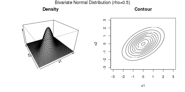
 Density and contour plot of a Bivariate Gaussian Distribution
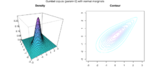 Density and contour plot of two Normal marginals joint with a Gumbel copula
Sklar's theorem[2] provides the theoretical foundation for the application of copulas. Sklar's theorem states that a multivariate cumulative distribution function
of a random vector
with margins can be written aswhere C is a copula.
The theorem also states that, given H, the copula is unique on
 , which is the cartesian product of the ranges of the marginal cdf's. This implies that the copula is unique if the margins Fi are continuous.
The converse is also true: given a copula
and margins Fi(x) then  defines a d-dimensional cumulative distribution function.
Fréchet–Hoeffding copula bounds
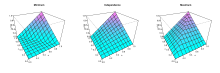 Graphs of the bivariate Fréchet–Hoeffding copula limits and of the independence copula (in the middle).
The Fréchet–Hoeffding Theorem (after Maurice René Fréchet and Wassily Hoeffding [3]) states that for any Copula
and any ![(u_1,\dots,u_d)\in[0,1]^d](3/583414790cdcaf5092ba81d83ab6c7e6.png) the following bounds hold:
the following bounds hold:The functions W is called lower Fréchet–Hoeffding bound and is defined as
The function M is called upper Fréchet–Hoeffding bound and is defined as
The upper bound is sharp: M is always a copula, it corresponds to comonotone random variables.
The lower bound is point-wise sharp, in the sense that for fixed u, there is a copula
 such that
  . However, W is a copula only in two dimensions, in which case it corresponds to countermonotonic random variables.
In two dimensions, i.e. the bivariate case, the Fréchet–Hoeffding Theorem states
Families of copulas
Gaussian copula
 Cumulative and density distribution of Gaussian copula with ρ = 0.4
The Gaussian copula is constructed by projecting a multivariate normal distribution on
 by means of the probability integral transform to the unit cube [0,1]d.
For a given correlation matrix
 , the Gaussian copula with parameter matrix Σ can be written as
where Φ − 1 is the inverse cumulative distribution function of a standard normal and ΦΣ is the joint cumulative distribution function of a multivariate normal distribution with mean vector zero and covariance matrix equal to the correlation matrix Σ.
The density can be written as [4]
where
 is the identity matrix.
Archimedean copulas
Archimedean copulas are an associative class of copulas. Most common Archimedean copulas admit an explicit formula for the C, something not possible for instance for the Gaussian copula. In practise, Archimedean copulas are popular because they allow to model dependence in arbitrarily high dimensions with only one parameter, governing the strength of dependence.
A copula C is called Archimedean if it admits the representation
where ψ is the so called generator.
The above formula yields a copula if and only if
 is d-monotone on
  . [5] That is, if the kth derivatives of satisfy
for all
 and
and  and ( − 1)d − 2ψd − 2(x) is nonincreasing and convex.
The generators in the following table are the most popular ones. All of them are completely monotone, i.e. d-monotone for all
 .
.Table with the most important generators[6] name generator 
generator inverse 
parameter Ali-Mikhail-Haq 


Clayton[7] 


Frank 

Gumbel 


Independence 

Joe 

Empirical copulas
When studying multivariate data, one might want to investigate the underlying copula. Suppose have observations
from a random vector
with continuous margins. The corresponding "true" copula observations would beHowever, the marginal distribution functions Fi are usually not known. Therefore, one can construct pseudo copula observations by using the empirical distribution functions
instead. Then, the pseudo copula observations are defined as
The corresponding empirical copula is then defined as
The components of the pseudo copula samples can also be written as
 , where
  is the rank of the observation
  :
:Therefore, the empirical copula can be seen as the empirical distribution of the rank transformed data.
Monte Carlo integration for copula models
In statistical applications, many problems can be formulated in the following way. One is interested in the expectation of a response function
 applied to some random vector
  .[8] If we denote the cdf of this random vector with H, the quantity of interest can thus be written as
If H is given by a copula model, i.e.,
this expectation can be rewritten as
In case the copula C is absolutely continuous, i.e. C has a density c, this equation can be written as
If copula and margins are known (or if they have been estimated), this expectation can be approximated through the following Monte Carlo algorithm:
- Draw a sample
 of size n from the copula C
 - By applying the inverse marginal cdf's, produce a sample of by setting

- Approximate
![\mathbb{E}\left[g(X_1,\dots,X_d)\right]](5/f455cdc78683e78640d1631e1d0e0f09.png) by its empirical value:
by its empirical value:
Applications
Quantitative finance
The applications of copulas in quantitative finance are numerous, both in the real-world probability of risk/portfolio management and in the risk-neutral probability of derivatives pricing.
In risk/portfolio management, copulas are used to perform stress-tests and robustness checks: panic copulas are glued with market estimates of the marginal distributions to analyze the effects of panic regimes on the portfolio profit and loss distribution. Panic copulas are created by Monte Carlo simulation, mixed with a re-weighting of the probability of each scenario.[9]
As far as derivatives pricing is concerned, dependence modelling with copula functions is widely used in applications of financial risk assessment and actuarial analysis – for example in the pricing of collateralized debt obligations (CDOs).[10] Some believe the methodology of applying the Gaussian copula to credit derivatives to be one of the reasons behind the global financial crisis of 2008–2009.[11][12] Despite this perception, there are documented attempts of the financial industry, occurring before the crisis, to address the limitations of the Gaussian copula and of copula functions more generally, specifically the lack of dependence dynamics[clarification needed] and the poor representation of extreme events.[13] There have been attempts to propose models rectifying some of the copula limitations.[13][14][15]
While the application of copulas in credit has gone through popularity as well as misfortune during the global financial crisis of 2008–2009,[16] it is arguably an industry standard model for pricing CDOs. Less arguably, copulas have also been applied to other asset classes as a flexible tool in analyzing multi-asset derivative products. The first such application outside credit was to use a copula to construct an implied basket volatility surface,[17] taking into account the volatility smile of basket components. Copulas have since gained popularity in pricing and risk management [18] of options on multi-assets in the presence of volatility smile/skew, in equity, foreign exchange and fixed income derivative business. Some typical example applications of copulas are listed below:
- Analyzing and pricing volatility smile/skew of exotic baskets, e.g. best/worst of;
- Analyzing and pricing volatility smile/skew of less liquid FX[clarification needed] cross, which is effectively a basket: C = S1/S2 or C = S1*S2;
- Analyzing and pricing spread options, in particular in fixed income constant maturity swap spread options.
Civil engineering
Recently, copula functions have been successfully applied to the database formulation for the reliability analysis of highway bridges, and to various multivariate simulation studies in civil, mechanical and offshore engineering.[citation needed]
Medicine
Copula functions have been successfully applied to the analysis of spike counts in neuroscience [19]
Weather research
Copulas have been extensively used in climate and weather related research.[20]
References
- ^ Nelsen, Roger B. (1999), An Introduction to Copulas, New York: Springer, ISBN 0387986235
- ^ Sklar, A. (1959), "Fonctions de répartition à n dimensions et leurs marges", Publ. Inst. Statist. Univ. Paris 8: 229–231
- ^ "J J O'Connor and E F Robertson" (March 2011). "Bigraphy of Wassily Hoeffding". School of Mathematics and Statistics, University of St Andrews, Scotland. http://www-history.mcs.st-andrews.ac.uk/Biographies/Hoeffding.html. Retrieved 8 November 2011.
- ^ Philipp Arbenz (2011): "Bayesian Copulae Distributions, with Application to Operational Risk Management - Some Comments". Forthcoming in 'Methodology and Computing in Applied Probability'
- ^ McNeil, A. J. and Nešlehová, J. (2009), "Multivariate Archimedean copulas, d-monotone functions and l1-norm symmetric distributions", The Annals of Statistics, 37(5b), 3059–3097.
- ^ Jan Marius Hofert (2010): Sampling Nested Archimedean Copulas with Applications to CDO Pricing. Dissertation at the University of Ulm
- ^ David G. Clayton (1978), "A model for association in bivariate life tables and its application in epidemiological studies of familial tendency in chronic disease incidence", Biometrika 65, 141–151. JSTOR (subscription)
- ^ Alexander J. McNeil, Rudiger Frey and Paul Embrechts (2005) "Quantitative Risk Management: Concepts, Techniques, and Tools", Princeton Series in Finance
- ^ Meucci, Attilio (2011), "A New Breed of Copulas for Risk and Portfolio Management", Risk 24 (9): 122–126, http://symmys.com/node/335
- ^ Meneguzzo, David; Vecchiato, Walter (Nov 2003), "Copula sensitivity in collateralized debt obligations and basket default swaps", Journal of Futures Markets 24 (1): 37–70, doi:10.1002/fut.10110
- ^ Recipe for Disaster: The Formula That Killed Wall Street Wired, 2/23/2009
- ^ MacKenzie, Donald (2008), "End-of-the-World Trade", London Review of Books, 2008-05-08, http://www.lrb.co.uk/v30/n09/mack01_.html, retrieved 2009-07-27
- ^ a b Lipton, Alexander; Rennie, Andrew. Credit Correlation: Life After Copulas. World Scientific. ISBN 978-9812709493.
- ^ Donnelly, C; Embrechts, P, (2010). The devil is in the tails: actuarial mathematics and the subprime mortgage crisis. ASTIN Bulletin 40(1), 1–33
- ^ Brigo, D; Pallavicini, A; Torresetti, R (2010). Credit Models and the Crisis: A Journey into CDOs, Copulas, Correlations and dynamic Models. Wiley and Sons
- ^ Jones, Sam (April 24, 2009), "The formula that felled Wall St", Financial Times, http://www.ft.com/cms/s/2/912d85e8-2d75-11de-9eba-00144feabdc0.html
- ^ Qu, Dong, (2001). "Basket Implied Volatility Surface". Derivatives Week, (4 June.)
- ^ Qu, Dong, (2005). "Pricing Basket Options With Skew". Wilmott Magazine (July.)
- ^ Onken, A; Grünewälder, S; Munk, MH; Obermayer, K (2009), Aertsen, Ad, ed., "Analyzing Short-Term Noise Dependencies of Spike-Counts in Macaque Prefrontal Cortex Using Copulas and the Flashlight Transformation", PLoS Computational Biology 5 (11): e1000577, doi:10.1371/journal.pcbi.1000577, PMC 2776173, PMID 19956759, http://www.ploscompbiol.org/article/info%3Adoi%2F10.1371%2Fjournal.pcbi.1000577
- ^ Schölzel, C.; Friederichs, P. (2008). "Multivariate non-normally distributed random variables in climate research – introduction to the copula approach". Nonlinear Processes in Geophysics 15 (5): 761. doi:10.5194/npg-15-761-2008.
Further reading
- The standard reference for an introduction to copulas. Covers all fundamental aspects, summarizes the most popular copula classes, and provides proofs for the important theorems related to copulas
-
- Roger B. Nelsen (1999), "An Introduction to Copulas", Springer. ISBN 978-0387986234
- A book covering current topics in mathematical research on copulas:
-
- Piotr Jaworski, Fabrizio Durante, Wolfgang Karl Härdle, Tomasz Rychlik (Editors): (2010): "Copula Theory and Its Applications" Lecture Notes in Statistics, Springer. ISBN 978-3-642-12464-8
- A paper covering the historic development of copula theory, by the person associated with the "invention" of copulas, Abe Sklar.
-
- Abe Sklar (1997): "Random variables, distribution functions, and copulas – a personal look backward and forward" in Rüschendorf, L., Schweizer, B. und Taylor, M. (eds) Distributions With Fixed Marginals & Related Topics (Lecture Notes – Monograph Series Number 28). ISBN 978-0940600409
- The standard reference for multivariate models and copula theory in the context of financial and insurance models
-
- Alexander J. McNeil, Rudiger Frey and Paul Embrechts (2005) "Quantitative Risk Management: Concepts, Techniques, and Tools", Princeton Series in Finance. ISBN 978-0691122557
External links
Categories:- Actuarial science
- Multivariate statistics
- Statistical dependence
- Systems of probability distributions

![C(u_1,u_2,\dots,u_d)=\mathbb{P}[U_1\leq u_1,U_2\leq u_2,\dots,U_d\leq u_d]](e/71e8b0dca72f1c2a0c7a16615b0002dc.png)

![C(u_1,u_2,\dots,u_d)=\mathbb{P}[X_1\leq F_1^{-1}(u_1),X_2\leq F_2^{-1}(u_2),\dots,X_d\leq F_d^{-1}(u_d)]](f/acf8bbb028d6a39ec16aa00c9de8ba3a.png)


![H(x_1,\dots,x_d)=\mathbb{P}[X_1\leq x_1,\dots,X_d\leq x_d]](1/3716e91b7885baab1ce598e7a4602198.png)


![\mathbb{E}\left[g(X_1,\dots,X_d)\right]=\int_{\mathbb{R}^d}g(x_1,\dots,x_d)\mathrm{d}H(x_1,\dots,x_d).](8/478ab73c146a46c22f9f8b8e0431e5d1.png)

![\mathbb{E}\left[g(X_1,\dots,X_d)\right]=\int_{[0,1]^d}g(F_1^{-1}(u_1),\dots,F_d^{-1}(u_d))\mathrm{d}C(u_1,\dots,u_d).](8/788aba48502c646d42fcf3b25c7035e4.png)
![\mathbb{E}\left[g(X_1,\dots,X_d)\right]=\int_{[0,1]^d}g(F_1^{-1}(u_1),\dots,F_d^{-1}(u_d))c(u_1,\dots,u_d)\mathrm{d}u_1\cdots\mathrm{d}u_d.](b/2cb9c87b420d0f5facaa756f65b40425.png)
![\mathbb{E}\left[g(X_1,\dots,X_d)\right]\approx \frac{1}{n}\sum_{k=1}^n g(X_1^k,\dots,X_d^k)](e/8bea27ac4d61a6a4b3325ea50b036498.png)
Wikimedia Foundation. 2010.